2 History of Past Cold and Warm Periods
Reconstructed solar activity shows ~5 deep minima and ~4 sustained maxima since antiquity, each tracking documented climate and societal impact.
2.1 Cosmogenic Isotopes as a Solar Proxy
To reconstruct solar activity beyond the brief era of direct observation, scientists rely on cosmogenic isotopes that serve as natural archives of cosmic-ray flux. [44] Among these proxies, Beryllium-10 (\(^{10}\)Be) concentrations are measured in Greenland ice cores such as Dye-3. These ice cores provide a continuous record of atmospheric deposition, allowing researchers to trace variations in solar modulation over millennia. [56][57][58][59][60][61] The precision of these records is crucial for understanding the long-term behavior of the Sun and its impact on Earth’s climate system. [62]
The production of beryllium-10 (\(^{10}\)Be) in the atmosphere serves as a sensitive recorder of solar modulation, particularly because the solar wind’s magnetic field shields Earth from galactic cosmic rays. [59] When solar activity is high, this shielding effect is enhanced, reducing the flux of cosmic-ray protons that generate \(^{10}\)Be. [59] For instance, high-resolution records from Law Dome ice in East Antarctica show a highly significant correlation (\(r_{xy}=0.64\)) between \(^{10}\)Be concentrations and neutron monitor data, which directly measures cosmic-ray intensity. [63] Furthermore, comparisons with the Greenland Ice Core Project data reveal that \(^{10}\)Be time series can differentiate between the strengths of solar minima even when sunspot numbers drop to near zero, such as during the Maunder Minimum. This sensitivity confirms that \(^{10}\)Be provides a continuous record of the open solar magnetic field, independent of the threshold effects that obscure sunspot observations during grand minima. [59] Thus, the cosmogenic isotope record faithfully registers solar centennial variability, offering a critical tool for understanding long-term solar-climate interactions beyond the limited span of direct sunspot observations.
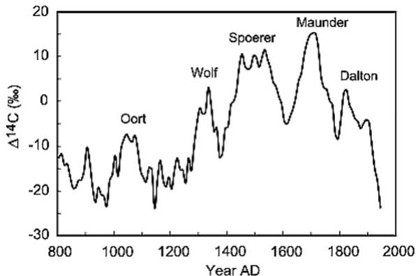
Ice-core archives from Antarctica and Greenland preserve beryllium-10 (\(^{10}\)Be), a cosmogenic isotope whose atmospheric production is modulated by solar activity. [34] These temperature anomalies, derived from various paleoclimate records, show a remarkable correlation with cosmic-ray variations inferred from isotopic data. [64] The resulting \(^{14}\)C production rate (p \(^{14}\)C) reflects the flux of incoming cosmic ray particles, which are modulated by the solar magnetic field. [65] This inverse relationship establishes \(^{14}\)C production rates as a robust indicator of solar variability. [66] For instance, the maximum \(^{14}\)C production rate in the last millennium occurred between AD 1645 and 1715, coinciding with the Maunder Minimum when sunspots were almost lacking. [33] In contrast, \(^{14}\)C concentration in tree rings can be influenced by changes in the global carbon cycle, complicating the isolation of solar signals. The first principal component explains 69% of the total variance, implying that \(^{14}\)C production changes throughout the Holocene are very similar to the \(^{10}\)Be changes found in polar ice cores from two different hemispheres. [56] Simulations starting at 500 BC using \(^{10}\)Be-derived production from Antarctic ice show a good match with IntCal04 atmospheric \(^{14}\)C variations in both amplitude and phase, with correlation coefficients (\(r^2\)) close to 0.9. [67] Consequently, long-term reconstructions rely on proxy evidence from natural archives, specifically cosmogenic isotope concentrations preserved in dendrochronologically dated tree rings and ice cores. Among these proxies, Carbon-14 (\(^{14}\)C) isotopes are extracted from ancient tree rings for solar proxy analysis, providing a reliable archive of past solar activity on time scales of years to centuries and millennia. This radiocarbon record establishes that radiocarbon production in the atmosphere, and consequently in tree rings, is owing to a cosmic ray flux which has significantly varied, being in inverse relationship with solar activity. [68][69][70][71] The longest and most precise annual \(^{14}\)C dataset, created by Brehm et al. using 13 oak timbers from buildings in the UK and Switzerland covering the period 969–1933 CE, demonstrates the persistence of the 11-year Schwabe cycle throughout the last millennium. [69] These annually resolved paleoclimatic and solar proxies from the same calendar-dated tree-ring sequence confirm a direct influence of the Schwabe cycle on climate, reaffirming that \(^{14}\)C in tree-ring chronologies can provide robust information on solar variability. [69] Furthermore, the regularity of longer cycles, such as the 178.7-year cycle, is sometimes disturbed, with patterns of solar minima like the Spörer and Maunder types recurring in steps of approximately 2402 years. By correcting for obfuscating variables such as the strength of the geomagnetic field, a function called the solar modulation potential is derived, which reveals the activity of the Sun over time via changes in cosmogenic isotope production. [68] This method confirms that the radiocarbon record in tree rings provides a reliable archive of past solar activity, allowing researchers to reconstruct solar behavior far beyond the reach of instrumental records. [44]
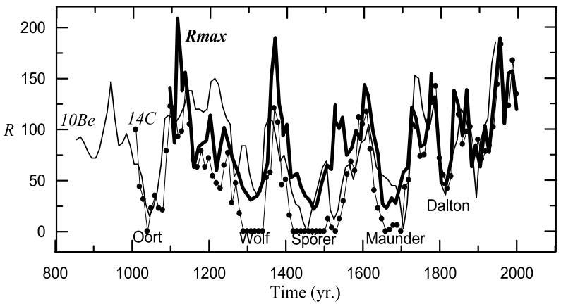
This figure displays a time series of reconstructed solar activity from 800 to 2000 CE, showing annual sunspot numbers derived from radiocarbon (¹⁴C, solid dots) and beryllium-10 (¹⁰Be, thin line) dat
2.2 Pre Maunder Grand Minima
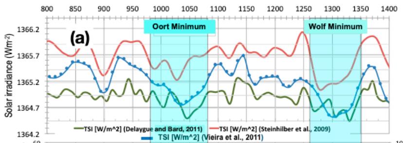
This period of reduced solar activity is further corroborated by auroral records; continuous Chinese observations from 900 A.D. to 1200 A.D. indicate that auroral activity was relatively weak during 1010–1050 A.D., consistent with the grand minimum conditions of the Oort Minimum. [73] The lack of auroral evidence in “The Poetic Edda,” assembled in southern Norway between 1000 and 1100 A.D., also aligns with the reconstructed auroral zone and the weak solar activity characteristic of the Oort Minimum. [73]
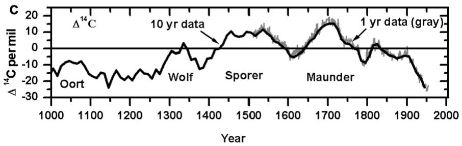
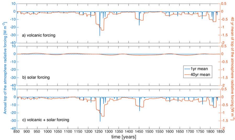
Solar activity reconstructions reveal distinct periods of prolonged low output, or grand minima, scattered across the historical record. [44] 1050, a signal inferred to indicate a period of minimum solar activity known as the Oort Minimum. This specific interval, spanning roughly from 1010 to 1070 or 1080, is identified in adjustment-free solar activity reconstructions as one of four grand minima since the year 1000 A.D., alongside the Wolf, Spörer, and Maunder events. The elevated \(\Delta^{14}C\) levels during this time confirm reduced solar modulation, as higher radiocarbon production corresponds to lower sunspot numbers in the inverted scale of the record. While some extratropical Northern Hemisphere temperature reconstructions do not explicitly highlight the Oort Minimum as a distinct cold anomaly, the cosmogenic isotope data establishes the solar quiescence. The timing of this minimum aligns closely with grand perihelion coincidences of Saturn, Uranus, and Neptune near the year 1050, suggesting a planetary association with Oort-type solar activity. These independent lines of evidence from radiocarbon dating and orbital mechanics suggest that the Oort Minimum was characterized by significantly reduced solar activity. Although the direct temperature signal in some proxy records is less pronounced than in later minima like the Maunder, the solar reconstruction confirms the event’s occurrence and duration. The consistency between the \(\Delta^{14}C\) peak and the solar activity reconstruction is consistent with the existence of this early grand minimum in the Holocene record. [32][19][2][67][74] The resulting \({}^{10}Be\) record spans approximately from year 840 AD to year 1980 AD, offering a near-decadal resolution with an average of 8 years per sample. [67] This resolution corresponds to a mean accumulation rate of about 7 cm water equivalent per year. [67] The reconstruction of \(\Phi\) — the solar modulation potential, a measure (in megavolts) of how strongly the heliospheric magnetic field shields Earth from incoming galactic cosmic rays — based on stacked records and a constant mixing scheme compares quite well with the one of McCracken et al. based on the South Pole record and their mixing model “M3” [67], with three marked differences. First, the Spörer Minimum corresponds to the weakest activity in our reconstruction, even after removing the lowest values around year 1456 AD. [67] Another important difference is a secondary maximum centered around year 1220 AD in the South Pole reconstruction, which does not exist at all in our stack. [67] A third important difference concerns the rank of the minima: in our stack the Spörer is the lowest minimum, followed by the Maunder, Wolf, Oort, and Dalton Minima, that is, the Oort and Maunder Minima are higher than in the McCracken et al. reconstruction. [67] The maximum of \(\Phi\) is found during the 20th century based on the raw \(\Phi\) values, but during the 8th century based on smoothed \(\Phi\) values. [67] As discussed in Sect. 3.3, trends in snow accumulation have probably biased the relative values of \(\Phi\) , and this would affect the rank of the reconstructed solar Minima and maxima. [67] In particular, the expected decrease in snow accumulation during the 16th and 17th centuries would have increased \(^{10}\mathrm{Be}\) concentration and biased \(\Phi\) towards lower values. [67] However, this bias would not (or less) apply to our reconstructed Spörer Minimum and would even lower the Maunder Minimum. Specifically, large volcanic eruptions caused short-term climatic effects, including cooler temperatures over several months due to reduced solar irradiation. This distinction is vital because stratospheric aerosols affect the global radiation budget by absorbing and, more importantly, backscattering incoming solar radiation, which causes a cooling of the lower atmosphere and the surface. [75][1][76] Statistical studies using superposed epoch analysis have identified a statistically significant average temperature decrease of about 0.2 to 0.5°C for 1 to 3 years following the times of known nineteenth and twentieth century eruptions. [75] However, this volcanic signal is transient; surface temperatures recover in a few years as the aerosols decay, meaning that volcanic forcing cannot account for the multi-decadal or centennial cooling trends observed during the Sumerian, Egyptian, or Roman minima. The volcanic signal expected in hemispheric or zonal surface temperature records in historical times is about the same as the background interannual variations in temperature, requiring careful compositing to isolate the signal from noise. [75] Therefore, when we observe sustained cooling periods that align with low solar activity in ¹⁰Be and ¹⁴C records, we are not looking at the aftermath of volcanic winters, which are brief and intense, but rather at the prolonged dimming of the Sun itself. Thus, the pre-Maunder record stands as a testament to solar dominance on decadal to centennial scales, independent of the short-term volcanic noise that punctuates the instrumental era.
2.3 The Maunder and Dalton Minima Up Close
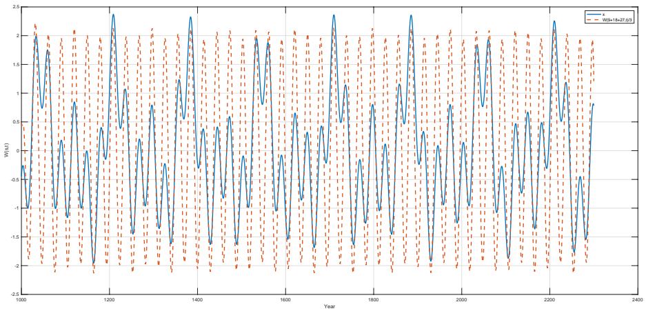
Furthermore, the cosmogenic record detects the Hallstatt 2,400-year cycle across the Holocene, suggesting a deep, rhythmic structure to solar output that predates the instrumented era.
Chapter 7 tells the Tambora story in full — the 1815 eruption, the ‘year without a summer,’ the failed harvests from New England to Finland. Here it is enough to note that the Dalton Minimum’s most infamous years were a volcanic exclamation point set inside an already sun-starved climate.
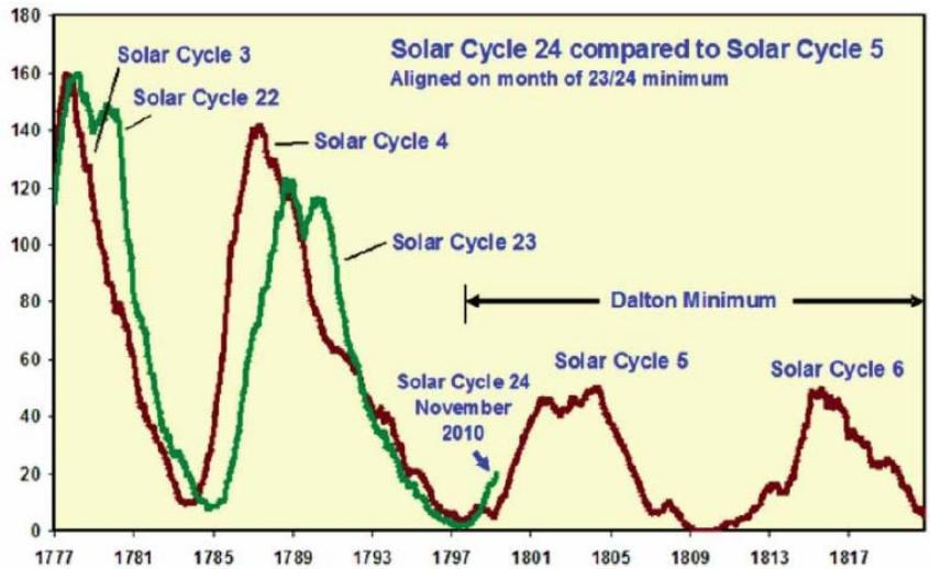
The Dalton Minimum was an active period for volcanic activity, a fact that highlights the complex interplay between solar and geological forcing during this era. [85] In addition to the massive Mount Tambora eruption, La Soufriere on Saint Vincent erupted in 1812. These concurrent events highlight how multiple geological disasters can compound cooling effects. [49][83] This overlap challenges simple attributions of climate change to a single driver, showing instead a period where solar hibernation and volcanic particulates likely worked in tandem to depress global temperatures. [86] The historical record thus suggests that the Dalton Minimum was not merely a solar phenomenon but a time of compounded climatic stress from both celestial and terrestrial sources. [87] Post described as the “last great subsistence crisis in the Western world.” As the sun went quiet during this interval, the Earth began to slowly cool, delaying the start of the planting season and limiting the harvest with early frost in the fall. [88] While modeling studies show a large range of simulated climate responses to solar forcings, with some attributing most cooling to volcanic effects, other analyses suggest solar cooling was a significant force for lower temperatures during the Dalton Minimum. For instance, Shindell et al. concluded that volcanic eruptions have rather strong but only short-lived effects on temperatures, while the reduction of the solar irradiance during the grand minimum affects temperatures on longer timescales. [88][85][46][1][49] Archibald (Australia), Duhau (Argentina), and Theodor Landscheidt (Germany) forecasted that the sun would enter a period similar to the Dalton Minimum or a more severe “Grand Minimum” in Solar Cycle 25 — within the 2020–2053 window this book adopts. [89] These forecasts underscore the potential for future solar minima to impact global temperatures and societal stability, echoing the severe conditions of the Dalton era. [49] The combined effects of volcanic eruptions and solar irradiance decrease could significantly modify global mean temperatures, with Wagner and Zorita showing modifications by up to several tenths of a degree. [85] However, the exact solar forcing used in some modeling studies remains unknown, highlighting the complexity of isolating solar impacts from other climatic factors.
2.4 Grand Maxima and Societal Abundance
Rather than a monolithic warming trend, the region experienced a distinct seesaw of precipitation conditions between the western and eastern basins, where the west often faced arid conditions during positive North Atlantic Oscillation periods, while the east sometimes experienced more humid conditions despite the broader NAO impact. [92] This regional divergence was driven by the interplay of multiple climate patterns, including the North Sea-Caspian Pattern, defined by the pressure difference between the North Sea and the Caspian Sea, which brought cool and dry winter conditions to the central and eastern Mediterranean when positive, and warm and wet conditions when negative. [92] Furthermore, the influence of a strong Siberian High could channel unusually cold airflow from Inner Eurasia into the eastern Mediterranean and the Middle East, contributing to rare phenomena such as snowfall and frost in Baghdad, events that were described several times during the Oort Minimum of the 11th century. These specific meteorological dynamics demonstrate that the Medieval Climate Anomaly in the Eastern Mediterranean was spatially and temporally incoherent, punctuated by recurring anomalies. Such variability underscores the necessity of examining regional climate drivers rather than relying on hemispheric averages, as local socio-political dynamics in the Byzantine Empire were likely shaped by these fluctuating environmental conditions rather than a steady thermal trend. [92][93] Elena Xoplaki and co-authors combined evidence of economic and demographic growth in Byzantium between 850 and 1300 CE with new findings from palynology, alongside documentary textual evidence and natural proxies for the Balkans and Asia Minor. [92] Their analysis identified potential links between climatic and societal changes, specifically noting correlations between a long-term trend towards wetter conditions in western Anatolia around AD 850–1000 and stable, relatively warm-wet conditions in northern Greece during AD 1000–1100. [92] Based on a marine record from the Athos basin in Northern Greece, they reconstructed changes in sea surface temperatures and other palaeoenvironmental factors. [92] Their data suggests a cooling trend from ca. [94] 500 to 850 CE, followed by a warming trend from ca. [92] 850 to 950 CE in the Northern Aegean. [92]
Palynological data, specifically pollen records from Asia Minor and the Southern Balkans, confirm a significant increase in agricultural cultivation across the Byzantine Empire beginning in the late 9th and 10th centuries, following a notable decline between the 6th and 8th centuries. [92] This expansion included intensified production of cerealia, olives, and wine, alongside shifts toward pasturage and animal husbandry, reflecting regional variations in land use. [92] Alexander Olson’s study on oak and olive cultivation in the middle Byzantine period demonstrates that this economic upsurge and agricultural intensification were consequences of greater pressure for surplus from elite figures, rather than demographic growth alone. [92] The data shows that modest landscape modifications and slow agricultural growth characterized the 10th and 11th century Aegean provinces, with more significant economic dynamics emerging only in the late 11th century. [92] This later period was driven by a Komnenian-led Byzantine state demanding higher tax revenue, an emerging class of big landowners seeking rent, and Italian merchants trading across the Aegean’s waters, which pressured peasants to produce a surplus that garnered coins on the market. [92] In 1069, for instance, the winter in Germany was harsh and long, causing rivers to freeze and leading to a significant shortage of wine and fruit due to the extreme cold. [40] These concurrent extremes demonstrate the global reach of climatic anomalies during this period. [3] In England, the year 1069 saw a great dearth, exacerbated by Norman conquests, where peasants resorted to cannibalism and sold themselves into slavery to survive. [40]
The Oort Solar Minimum (ca. 1010–1080) was characterized by reduced solar activity and cooler global average temperatures. An adjustment-free reconstruction of the solar activity over the last three millennia confirms four Grand minima since the year 1000A.D, including the Oort (1010–1070) period. The smoothed reconstruction — built from tree-ring data by ensemble empirical mode decomposition with variance matching — exhibited a general agreement with the variation of the reconstructed total solar irradiance, with a significant correlation (r = 0.498, edf = 34, p<0.01) during the common period 849–2000 AD. The relatively cold conditions between the two warm peaks around AD 1000 and 1100 seemed to be related to the Oort Minimum. Several of the periods with especially low solar activity are also visible in the reconstruction, such as the Wolf Minimum (c. [19][95][2][96] This complex climatic backdrop did not necessarily cause societal collapse in Byzantium or neighbouring polities; instead, it appears to be consistent with long-term economic expansion for certain times, suggesting that the empire possessed significant resilience against exogenous shocks. [92] A detailed examination of the winter of 927–28 illustrates this dynamic clearly. [92] Rather, the long winter was later connected with what the state and the peasants perceived as a socioeconomic crisis, serving as a lens through which contemporaries understood the reasons for social transformation. [97] The environmental stressor, even if it was not the harshest winter of the tenth century in physical terms, impinged upon the complex web of crop ecologies, social relations, and the state’s interests. [97] It added new momentum to extant social dynamics, specifically the trend of office-holding elites accumulating wealth to become an increasingly powerful social group. [92] While Byzantine society as a whole proved resilient, surviving the crisis, the price for this resilience was a significant shift in the balance of socioeconomic relations. [97] The winter offered an opportunity for the more affluent to exploit peasants whose livelihoods depended on ecological niches incapable of withstanding prolonged cold spells. [97] Thanks to buffers such as existing estates, accumulated gold, and local connections, elite groups could exploit local subsistence crises across the provinces to improve their situation relative to both the producing population and the state. [97] This suggests that environmental stressors stimulated social evolution rather than causing direct collapse. [97] Recent regional studies, including pollen data from Lake Belevi and Bafa Gölü, alongside written records like the 1073 charter for Andronikos Dukas regarding flood-damaged estates in the Maeander delta, support this nuanced view. [92] These archives inform us about short-term localised events and long-term trends, allowing for a more detailed description of the resilience of rural and urban communities. [92]
2.5 The Long Cycles Hallstatt Eddy Bray
This perspective raises serious concerns about a coming ice age in several thousand years, rather than catastrophic warming from greenhouse gas emissions on the timescale of the 21st century. [8] If Vinós’ analysis is correct, the belief that we can control Earth’s climate by reducing CO₂ emissions may turn out to be the greatest folly of the 21st century, underscoring the need for a broader debate on the true drivers of climate change. [1]
Climate models employing reductions in total solar irradiance of 0.4%, 0.25%, 0.12%, and 0.08% indicate that even a ‘grand’ minimum state would only partly reduce global mean temperature by 0.1 K, or delay the projected rise. [98] More moderate scenarios result in an even weaker signal, while recent experiments with a 0.12% reduction apportioned across the spectrum, or a larger 0.85% reduction in UV irradiance alone, show regional responses in the Northern Hemisphere that do not appear to scale linearly with the forcing magnitude. [98] These simulations suggest that a hypothetical grand solar minimum would offset only approximately 0.2 K of anthropogenic warming. Consequently, such a solar downturn is unlikely to significantly alter the long-term warming trend driven by greenhouse gas emissions. [99] These higher estimates imply that solar forcing could be important for climate variability, particularly if the irradiance from the quiet Sun varies significantly over time. [100] Some studies utilizing these high solar variability TSI estimates argue that solar forcing dominated long-term warming since the 19th century, suggesting that the solar contribution to observed temperature increases may be larger than previously thought. [101] Consequently, the relative importance of solar forcing in recent warming trends continues to be a subject of significant scientific debate.
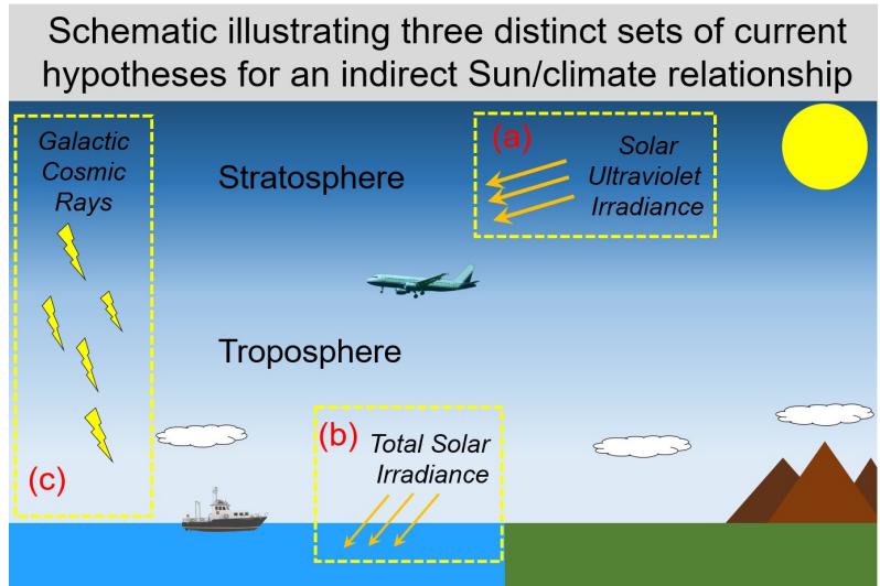
Solar forcing of Earth’s climate operates through both direct and indirect processes, with the simplest direct mechanism involving variations in solar radiative output. [102] While currently believed too small to have had a dominant influence on surface climate, variations in solar irradiance may have been larger back in time. [103] Indirect effects include solar-induced changes in atmospheric transparency influencing the radiative budget of the planet. [102] One possibility is that changes in the solar output of ultraviolet (UV) radiation affects temperatures in the stratosphere through absorption by ozone, which has the potential to influence the large-scale dynamics of the troposphere. [102] During solar maxima, the energy in the UV spectrum can be several percent higher than during solar minima. [64] Consequently, while solar variability contributes to natural climate fluctuations, it is generally considered a minor factor compared to anthropogenic greenhouse gas emissions.
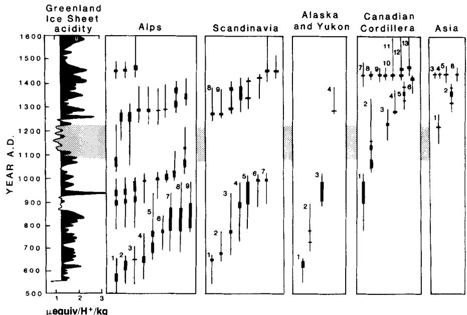
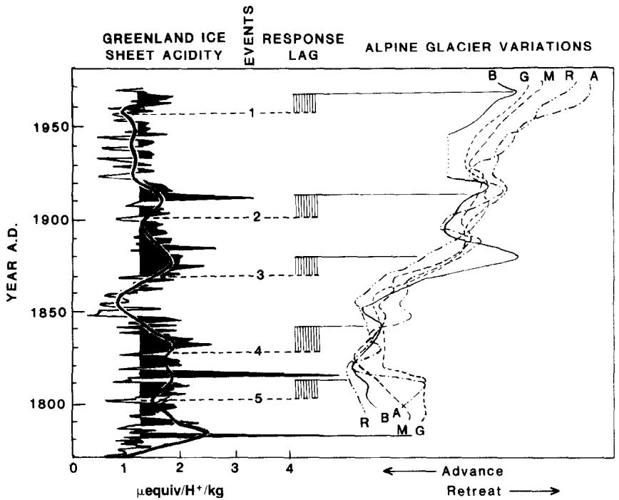
Porter demonstrates that sulfur-rich aerosols generated by volcanic eruptions are a primary forcing mechanism of glacier fluctuations and climate on a decadal scale, suggesting volcanic impacts as a dominant driver of interannual-to-decadal Northern Hemisphere temperature variability. The study shows that episodes of glacier advance consistently associate with intervals of high average volcanic aerosol production, inferred from acidity variations in a Greenland ice core. [104][79][56] Specifically, advances occur whenever acidity levels rise sharply from background values to reach concentrations \(\geqslant1.2\ \mu equiv\ H^{+}/kg\) above background. [104] A phase lag of about 10–15 yr, equivalent to reported response lags of Alpine glacier termini, separates the beginning of acidity increases from the beginning of subsequent ice advances. [104] The amount of surface cooling attributable to individual large eruptions or episodes of eruptions is similar to the probable average temperature reduction during these advances, ca. \(0.5^{\circ}-1.2^{\circ}C\), as inferred from depression of equilibrium-line altitudes. [104] This climatic shock coincided with the political transition from the Roman Republic and Ptolemaic Kingdom to the Roman Empire, a period marked by unusual climate, crop failures, famine, disease, and unrest in the Mediterranean, suggesting significant vulnerability to hydroclimatic shocks in ancient states. These findings imply that such environmental stressors may have exacerbated existing political tensions, potentially accelerating the collapse of established regimes. [105][106][107][108]
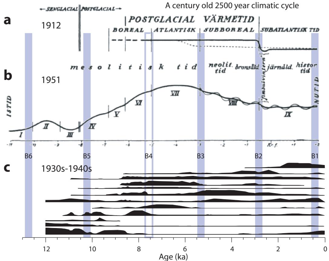
Model simulations using the MPI-ESM-P ensemble suggest an abrupt weakening of the subpolar gyre around 1600, driven by anomalous Arctic freshwater export into the Labrador Sea. This shift, observed in the Past1000-R3 simulation, indicates a reduction in gyre strength of 0.72 Sv over two decades, separating two stationary regimes. [26][27] The mechanism appears to be stabilized by positive feedbacks: reduced poleward heat transport cools the Nordic Seas, enhancing sea ice growth and export through the Denmark Strait, which further freshens the upper ocean. [26] These simulated changes, including expanded sea ice and reduced subpolar meridional heat transport, are consistent with paleoclimate reconstructions of Little Ice Age-type episodes, despite timing discrepancies attributed to internal climate variability. [26] Iversen to refine postglacial period zonation and establish a summer vegetation-based temperature scale for the Scandinavian Holocene by the 1940s. [1] These efforts produced Holocene climate reconstructions that closely mirror current understanding, revealing that the Holocene climate can be subdivided into periods of distinct climatic conditions, as illustrated in a diagram by Rutger Sernander from 1912. [1] The resulting vegetation stages allow for the distinction of a 2500-year vegetation and faunal cycle, with some botanists like Sernander proposing that transitions between periods were abrupt rather than gradual. [1] Specifically, Sernander linked the last transition between the Sub-Boreal and the Sub-Atlantic, occurring around 650 BC, to the “Fimbulvintern,” or Great Winter of the Sagas, which marks the end of the Nordic Bronze Age and rendered the Nordic countries a colder place. [1]