4 The Grand Solar Cycles: Zharkova’s Two-Wave Dynamo
Zharkova’s PCA of synoptic magnetograms reveals two magnetic waves whose beating predicts a Modern Grand Solar Minimum running ~2020–2053.
4.1 The Solar Background Magnetic Field
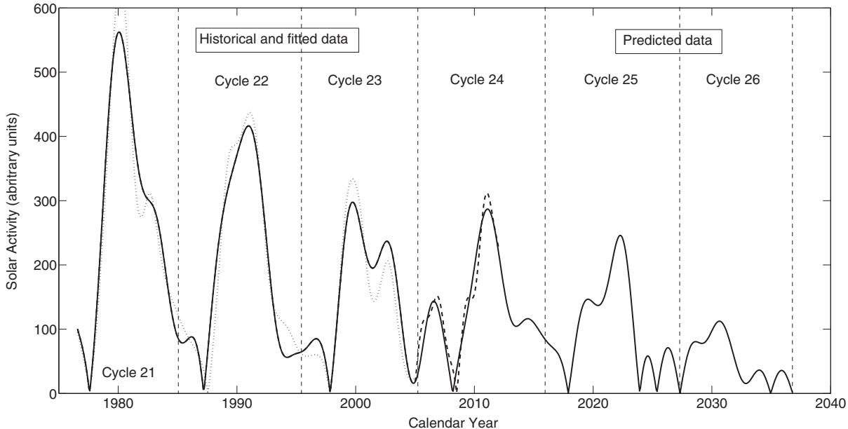
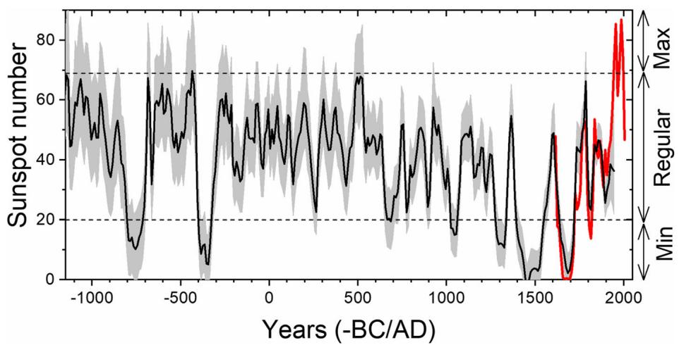
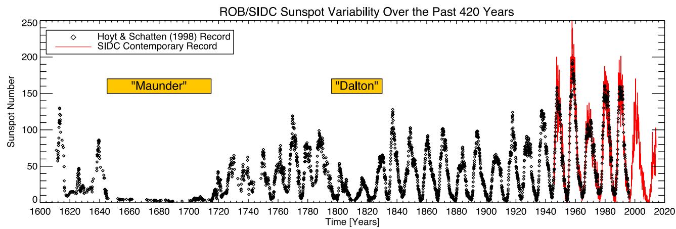
In contrast, the background field is measured across the full disk using synoptic magnetograms from observatories like the Wilcox Solar Observatory. Recent analyses have applied Principal Component Analysis (PCA) to these low-resolution full-disk solar background magnetic field measurements to derive the dominant eigenvalues that cover the maximum variance of the data. [160] This method identifies eigenvectors, or Principal Components (PCs), which come in pairs and reflect the main dipole dynamo waves produced by the solar dynamo mechanism. [161] By classifying these PCs using symbolic regression based on the Hamiltonian principle, researchers have derived mathematical formulae describing their amplitude and phase variations. [160] The summary curve of these two PCs, derived for cycles 21–23 and predicted for cycles 24–26, shows a noticeable decrease in predicted average sunspot numbers, linked to a reduction in the amplitudes and an increase in the phases of the principal components of the solar background magnetic field. [162] Furthermore, extending this prediction thousands of years backward and forward reveals the occurrence of a grand solar cycle of 350–400 years, successfully reproducing well-known historical events such as the Maunder, Wolf, Oort, and Homeric Grand Solar Minima.
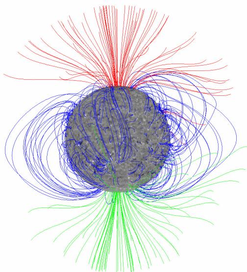
To isolate the large-scale solar background field from the chaotic noise of active regions, researchers rely on low-resolution magnetograms from the WSO Babcock solar magnetograph. [163] The Stanford University telescope, equipped with a 22.9m vertical Littrow spectrograph, has provided daily sun-as-a-star integrated light measurements of the mean solar magnetic field since May 1975. [164] The polarity pattern observed in these mean field measurements is essentially identical to the interplanetary magnetic field sector structure seen near Earth, albeit with a four-day lag. [164] These principal components, which come in pairs, are considered a reflection of the main dipole dynamo waves in the solar poloidal magnetic field produced by the dynamo mechanism. [160] By applying symbolic regression based on the Hamiltonian principle, scientists derived mathematical formulae describing the amplitude and phase variations of these eigenvectors. [160]
To isolate the solar background magnetic field from the noise of active regions, researchers applied principal component analysis to low-resolution full-disk synoptic magnetic maps measured by the Wilcox Solar Observatory. [165] This statistical technique decomposes the temporal variations of latitudinal magnetic waves into eigenvectors, each assigned to a separate process supported by its derived variance. [11] The analysis reveals that the eigenvalues and corresponding eigenvectors come in distinct pairs, with the first two eigenvalues covering 39% of the observed magnetic data variance and the next two covering 18%. [11] Collectively, these four pairs account for about 95% of the total magnetic data variance, suggesting that the solar background field is dominated by a small number of coherent modes rather than random fluctuations. These principal components, identified as the largest eigenvectors, represent the primary symmetric structures in the latitudinal distribution of the field. [11][128][166][167][168] This mathematical approach treats the magnetic field as potential between the photosphere and a source surface, where the field is presumed to be exactly radial. [168] The harmonic coefficients are generated based on summary year-long synoptic maps for every rotation, with a cadence equal to half a Carrington rotation. [169] The decomposition relies on the assumption that the magnetic field is potential between the photosphere and the source surface, while the field is presumed to be exactly radial at the source surface. [132] This technique allows for the precise extraction of the large-scale magnetic structure from the complex synoptic data. [129] The use of associated Legendre polynomials demonstrates that the solar surface magnetic field can be effectively broken down into its constituent harmonic parts. [132] The harmonic coefficients are derived from the synoptic maps, ensuring that the analysis is grounded in observational data. [169] These models rely on line-of-sight measurements of the photospheric magnetic field, which are mapped up to a hypothetical coronal source surface where the field is assumed to be purely radial. [168] This approach assumes that there are no currents in the corona between the photosphere and the source surface, meaning the curl of the magnetic field is zero. [168] By solving Laplace’s equation, the coronal field lines are determined, allowing for the classification of open flux that extends from the photosphere to the source surface. [168] However, the accuracy of these models is affected by several factors, including the assumption of time-invariance of the photospheric boundary and the challenge of resolving polar magnetic fields due to line-of-sight projection.
4.2 PCA and the Two Wave Decomposition
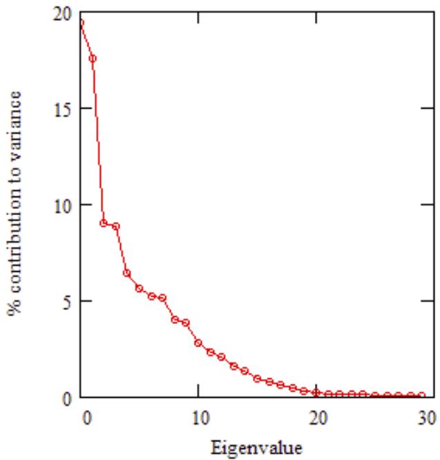
To distill the main parameters of the waves present in observational solar magnetic data, researchers applied Principal Component Analysis (PCA) to low-resolution full disk solar background magnetic field measurements. [160] This orthogonal linear transformation reduces multi-dimensional data to lower dimensions for analysis, ensuring that the greatest variance by any projection of the data lies on the first coordinate, known as the Principal Component (PC), with the second PC orthogonal to the first defined by the second largest variance. [160] The technique simultaneously reduces data dimensionality, increases signal-to-noise ratios, and orthogonalizes the resulting components so they can be ascribed to separate physical processes. [160] PCA was applied to the poloidal magnetic field data measured by the Wilcox Solar Observatory, which became available from cycle 21 to cycle 24 with an accuracy better than 0.5 Gauss. [160] By calculating the covariance matrix of the magnetic field data and its variance as the eigenvalues of magnetic oscillations, the analysis derived the eigenvalues of the Sun’s own magnetic oscillations. [161] The sets of eigenvalues and eigenvectors were derived from the observed magnetic synoptic maps and sorted by the variance of the data contributing to each eigenvector. [11] This process revealed that the eigenvalues and corresponding eigenvectors come in pairs, with the first two eigenvalues covering 39% of the observed magnetic data variance, the next two covering 18%, and all four pairs covering about 95% of the magnetic data variance. [11] The first pair of two largest eigenvalues, with the maximum variances of the data corresponding to the two largest eigenvectors, were considered to be the Principal Components. [160] These PCs are considered the main dipole dynamo waves of the solar poloidal magnetic field. [160] The PCA method uses the covariance matrix of the magnetic field data and its variance as the eigenvalues of magnetic oscillations, defining the magnetic wave properties as shown in the Scree plot. [161] Using PCA, researchers managed to derive the eigenvalues of the Sun’s own magnetic oscillations, showing clearly at least four noticeable pairs with large eigenvalues covering 96% of the total data variance. [161] The first two highest eigenvalues were used to build eigenvectors for the two principal components, or coherent magnetic waves, corresponding to these eigenvalues. [160] This is equivalent to deriving different wavelengths of white light after it is split in a prism. [150] Now these two magnetic waves can be assigned to unique physical processes. [161] By applying Parker’s model for two layers with meridional circulation, researchers derived that these PC waves correspond very closely to the waves generated by dipole magnetic sources. [160] Principal Component Analysis (PCA) of synoptic magnetic maps from cycles 21–24 yields eigenvectors that cover the majority of magnetic data variance. The leading eigenvectors are thus interpreted as coherent dipole dynamo waves, suggesting that the solar poloidal field is dominated by a small number of distinct physical modes. [11][160][161][165][163]
Principal Component Analysis of the low-resolution full disk solar background magnetic field, measured by the Wilcox Solar Observatory from synoptic full disk magnetic maps, isolates the dominant eigenvalues covering the maximum variance of the data. [160] The first pair of two largest eigenvalues, corresponding to the two largest eigenvectors, accounts for 39% of the observed magnetic data variance, while all four pairs cover about 95%. [170] Extrapolating these principal components backward reveals two 350-year grand cycles superimposed on the 22-year cycles, reproducing historical features such as the Maunder and Dalton minima. [160] This approach confirms that the interaction of dynamo waves with close frequencies leads to beating effects responsible for grand cycles, providing a confident prediction of solar activity on a millennium timescale. [160] These two principal components, covering about 39% of the variance of the whole magnetic field data, are found originating in opposite hemispheres and travelling with an increasing phase shift, defining the active hemisphere for odd and even cycles. [160] This stability reassures the health of the dynamo machine, while variations in wave frequencies cause a beating effect that produces grand cycles and grand minima occurring every 350–400 years. [171]
Principal Component Analysis applied to low-resolution full disk solar background magnetic field data from the Wilcox Solar Observatory reveals that eigenvalues and corresponding eigenvectors emerge in pairs, with the first two accounting for 39% of the observed magnetic data variance and the first four pairs covering approximately 95%. [11] However, converting the resulting eigenvector summary curve into a modulus summary curve is necessary to detect the 11-year solar cycle, as the raw eigenvector data alone does not clearly resolve this periodicity without such transformation. This mathematical step ensures that the oscillatory nature of the magnetic waves is properly captured, allowing the superposition of these principal components to reconstruct the historical sunspot envelope and predict future solar activity minima. [132][11][166][160][171]
Principal Component Analysis of the low-resolution full-disk solar background magnetic field, measured by the Wilcox Solar Observatory, isolates dominant eigenvalues that correspond to eigenvectors reflecting the main dipole dynamo waves in the solar poloidal magnetic field. [160]
The decomposition of solar magnetic data reveals that the Sun’s activity is not driven by a single oscillator, but rather by the superposition of multiple waves generated by distinct magnetic sources within the solar interior. [172] Theoretical evaluations indicate that the quadruple magnetic wave, originating in the inner layer at the bottom of the Solar Convective Zone, accounts for the occurrence of centennial oscillations in the summary curve of solar activity. [173] This mechanism supports the restoration of historical features such as the Dalton minimum at the beginning of the nineteenth century and another Gleissberg minimum at the start of the twentieth century, which were not fully captured by dipole-only models. [173] The beating effect between the dipole and quadruple waves naturally produces an envelope wave with a period of approximately 100 years, aligning with the observed centennial cycle. [161]
4.3 Isotope Validation
Studies such as those by Delaygue and Bard have examined Beryllium-10 records from Central Antarctica, specifically from the South Pole and Dome Fuji stations, covering the last millennium to quantify the relationship between ice-core deposition and production rates. [67] In contrast, ¹⁰Be offers a more direct proxy; as an aerosol-borne isotope, it is removed from the atmosphere relatively fast within a few years and stored in natural archives such as polar ice sheets. Because of its short atmospheric residence time, ¹⁰Be directly reflects cosmic ray intensity variations with almost no attenuation and a delay of only 1–2 years. [56]
The global carbon cycle imposes significant constraints on the resolution of solar activity records derived from radiocarbon. [176] Furthermore, the carbon cycle delays the response of atmospheric ¹⁴C concentration relative to production variations, creating a phase lag that ranges between 0 and 90°, with larger lags occurring for shorter periods. For centennial variations, this phase lag is approximately 45°, meaning atmospheric ¹⁴C concentration lags production by roughly 12 years. [67] This specific lag aligns with the delay estimated by Bard et al. between the South Pole ¹⁰Be record and the IntCal04 ¹⁴C record. [67] While 12-box models predict larger phase lags due to stratospheric transfer times, adequate observations remain lacking to fully validate these predictions. [67] Consequently, the uncertainty in reconstructed ¹⁴C due to carbon inventory remains a critical factor, with different box models showing varying attenuations and time lags that complicate the direct interpretation of high-frequency solar signals in tree-ring data.
Ice-core records of beryllium-10 (\(^{10}\)Be) provide a critical proxy for solar activity, as this isotope is produced by high-energy galactic cosmic-ray interactions with atmospheric oxygen and nitrogen. [177] Because the solar wind’s magnetic field deflects these cosmic rays, \(^{10}\)Be production rates are anti-correlated with solar activity, meaning higher sunspot numbers correspond to lower \(^{10}\)Be concentrations in polar ice. [177] To validate solar modulation models during the Maunder Minimum (1645–1715), researchers compared model results with \(^{10}\)Be observations from two independent ice cores, Dye3 and NGRIP, which are separated by more than 1000 km. [178] The NGRIP dataset, in particular, shows an inverted phase relation during the Maunder Minimum that was not employed in earlier studies, suggesting that the \(^{10}\)Be cycling observed during this grand minimum was indeed a solar modulation effect rather than a terrestrial artifact. This consistency between spatially separated ice-core proxies and sunspot reconstructions supports the reliability of using cosmogenic isotopes to hindcast solar variability and validate dynamo models. [178][177][179] For instance, simulated \(\Delta^{14}C\) levels have been found to deviate from IntCal04 data by several percent during specific centuries, often driven by anomalies in the South Pole or Dome Fuji \({}^{10}Be\) records. [67]
Cosmogenic isotopes such as beryllium-10 and carbon-14 serve as proxies for past cosmic-ray flux, offering a record that extends far beyond the era of neutron monitors. [148] Consequently, extracting the solar component from the ¹⁴C record becomes significantly more difficult for the modern period, as the anthropogenic trend competes with and often overwhelms the subtle variations driven by solar activity. Thus, the isotope validation section concludes that the two-wave model’s robustness is best confirmed in the pre-industrial record, where anthropogenic noise is absent, while the modern era requires careful deconvolution of fossil-fuel-induced isotopic shifts to assess the model’s accuracy.
4.4 The 2020 2053 Modern Grand Solar Minimum Prediction
Analysis of this double-dynamo system establishes that the Sun entered a modern Grand Solar Minimum in 2020, a period of reduced solar activity expected to last until 2053. This prediction is supported by multiple independent methodologies; for instance, Velasco Herrera et al. applied a Bayesian algorithm to averaged sunspot numbers and obtained similar results, reporting the modern Grand Solar Minimum to occur in cycles 25-27. [166][180][181] Furthermore, these prediction results were confirmed by other researchers, including Kitiashvili and Obridko et al., who utilized the same WSO synoptic magnetic field data to obtain spectra of the zonal harmonics of the solar background magnetic field approaching the Grand Solar Minimum, interpreting them with 3D solar dynamo models. The current quiet Sun is caused by a significantly reduced magnetic field generated by the interference of double dynamo magnetic waves, which means that during this Grand Solar Minimum, solar irradiance will be reduced by about 3 W/m², or 0.22%. [180] This reduction in solar irradiance caused by the Grand Solar Minimum effect works in opposition to the increase of solar irradiance caused by orbital solar inertial motion effects, creating a complex interplay of forcing mechanisms that define the thermal baseline for the coming decades. [180]
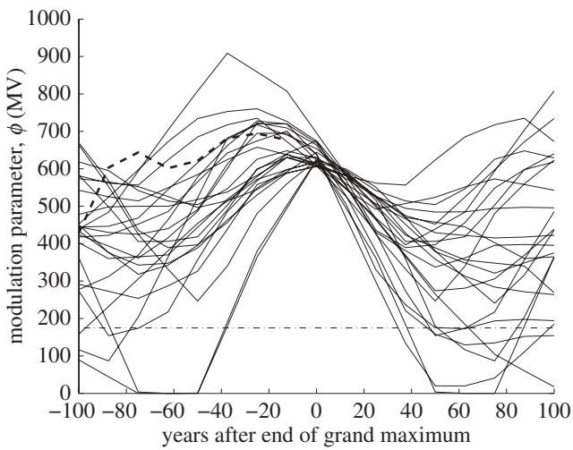
Statistical analysis of past grand maxima suggests a 1-in-12 probability of a Maunder-like grand minimum occurring within 50 years. This estimate derives from a superposed epoch analysis of the modulation parameter at the end of the previous grand solar maxima in the last 9300 years, based on the composite reconstruction of the modulation parameter from Steinhilber et al.. [182][181][166][156][183] Furthermore, Owens et al. created a data set for solar wind parameters dating back to 1617 to investigate Maunder minimum conditions and find the most probable coronal magnetic field configuration for this period. This configuration could be used for any past or future grand minima. [182]
Predicting the amplitude of solar cycles remains highly uncertain, with models for Cycle 24 showing wide disagreement. This uncertainty stems from the fact that cycle prediction is a fairly model-dependent affair, as evidenced by contradictory forecasts for Solar Cycle 24. [184][185][186][181] While Dikpati et al. predicted it would be the strongest cycle in fifty years, Choudhuri et al. concluded it would be the weakest in a century. [185] These divergent outcomes highlight that there are still many uncertainties in solar dynamo models, making it worthwhile to analyze the physical basis of solar cycle prediction carefully rather than having too much faith in predictions from any particular model. [131] The community-wide panels convened to construct consensus opinions on upcoming cycles often receive a broad range of submissions that cover almost all potential physically reasonable outcomes. [186] Consequently, the strength of every solar cycle a few years before its onset cannot be determined with precision, demonstrating the inherent difficulty in forecasting solar activity. Consequently, the modest irradiance decline predicted for the upcoming Modern Grand Solar Minimum implies a limited direct radiative cooling effect, consistent with the model results assuming small TSI variation.
The thermal implications of the predicted solar dimming are quantified through simple energy-balance calculations that relate changes in Total Solar Irradiance (TSI) to Earth’s effective temperature. [153] Taken at face value, the predicted ~3 W/m² (0.22%) drop in TSI works out — once spread over the spinning globe and corrected for reflection — to a direct radiative cooling of only one or two tenths of a degree: real, but modest. That is precisely why this book’s argument does not rest on irradiance arithmetic alone. The chapters that follow lay out the amplifiers — the cosmic-ray cloud seeding of Chapter 6, the volcanic coupling of Chapter 7 — that turn a two-tenths-of-a-degree nudge into Little Ice Age winters. Wherever this book quotes a larger cooling, it is a claim about that amplified response, not about the bare radiative term.
The solar activity became systematically decreasing from cycle 21, coinciding with a decrease of the solar background magnetic field in the approach of the grand solar minimum (GSM) (Zharkova et al. [181] 2015; Zharkova & Shepherd 2022). These prediction results about the modern GSM in cycles 25-27 were confirmed by some other researchers (Kitiashvili 2020; Obridko et al. [181] This long-term perspective, which incorporates both the historical sunspot number record covering the last 400 years and paleoreconstructions extending throughout the Holocene, provides critical observational constraints for dynamo models. [119]
4.5 Flare Physics the Same Magnetic Field
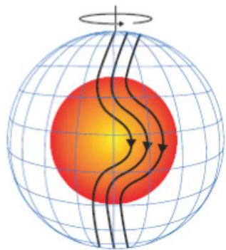
To understand the magnetic architecture that drives long-term solar variability, one must first anchor the analysis in the established physics of the solar dynamo, the engine that generates the 11-year Schwabe cycle. [44] The classical Parker model, proposed in 1955, demonstrates that this cycle arises from a self-exciting loop of magnetic field generation. [128] Furthermore, large-scale circulation patterns, such as the azimuthal rolls discovered by Ribes and Mein in 1984, modulate surface rotation and appear to regulate the internal shear that drives the dynamo.
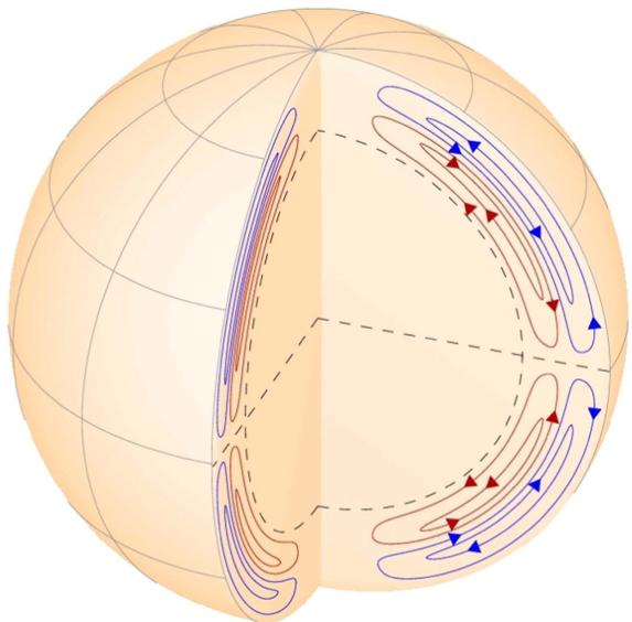
The Babcock–Leighton type dynamo models demonstrate that meridional circulation regulates the solar cycle period by transporting magnetic flux from the surface to the tachocline. This advective process is central to the flux transport dynamo framework, where the poloidal field generated by tilted bipolar regions is carried poleward and then downward to the tachocline. [185][189] The time scale of this circulation sets the dynamo period, establishing a direct link between flow speed and cycle length. [142] Models suggest that stochastic fluctuations in the alpha-effect cannot trigger grand minima, whereas a strong decrease in meridional circulation can. [189] Thus, the variability of this transport mechanism provides the physical basis for the irregularities seen in the solar record, connecting the large-scale dynamo operation to the potential for Maunder-like grand minima. [189]
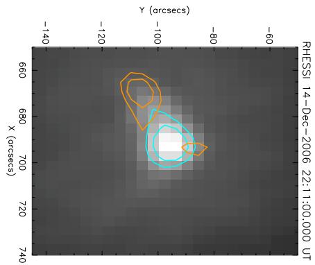
The irregular occurrence of grand minima observed in cosmogenic isotope records suggests that stochastic drivers in dynamo models are essential for reproducing long-term solar activity variability. Studies indicate that long-term fluctuations, including secular trends and extreme activity levels, originate from stochastic fluctuations in the driving parameters of the solar dynamo mechanism. [190][191][192][193][194] For instance, random fluctuations in the angular momentum transport process and the Babcock-Leighton mechanism generate grand minimum and maximum-like periods in fully non-linear flux-transport dynamo simulations. [192] Thus, the inclusion of stochastic drivers supports the understanding that grand minima are a special state of the solar dynamo, distinct from normal or high activity phases, driven by chaotic or random processes within the solar interior. By solving the time-dependent Fokker–Planck equation, the studies evaluate how electron beams precipitate into the solar atmosphere, revealing that magnetic convergence significantly alters energy deposition. [195] Thus, the flare work is not an isolated phenomenon but part of a unified research programme where the same magnetic field configurations that predict grand minima also dictate the intensity and depth of flare heating. Observations of the 23 July 2002 flare reveal that sharp temporal increases in hard X-ray emissions are closely correlated with variations in the photospheric magnetic field, particularly around the apparent magnetic neutral line. [196] Cross-correlation analysis of this event shows a noticeable positive correlation of 0.5–0.6 between temporal magnetic variations and HXR light curves, with a time lag no larger than 1–2 minutes across all energy bands. [197] These irreversible, steplike changes in magnetic flux, which reach a new steady state without returning to preflare values, demonstrate that magnetic field restructuring is responsible for initiating flare phenomena. [196] Observations of the 2006 December 14 X-class flare, utilizing GONG, Hinode, and RHESSI, revealed extended ribbon emission propagating through umbrae and penumbrae in both hemispheres, with energy deposition at the photospheric level occurring over a more confined area than the overlying chromosphere. [198] These measurements demonstrated asymmetries in hard X-ray source intensity and size between Northern and Southern ribbons, alongside strong impulsive changes in longitudinal magnetic flux at magnetic reversals. [198] Observations of the 23 July 2002 flare provide concrete evidence of this linkage, revealing that sharp temporal increases in hard X-ray (HXR) emissions are closely correlated in time with variations of the magnetic field measured in the photosphere. [196] Specifically, the magnetic flux change over the duration of this flare was approximately \(1.2 \times 10^{21}\) Mx, a significant alteration that occurred primarily around the apparent magnetic neutral line (AMNL). [196] Crucially, these magnetic field changes were found to be irreversible or steplike; the field reached a new level of steady state and did not return to its preflare value, a pattern consistent with theoretical expectations that irreversible magnetic changes are responsible for the initiation and development of flare phenomena. This connection is further strengthened by cross-correlation analysis, which shows a noticeable positive correlation of 0.5–0.6 between temporal magnetic variations covering the AMNL and HXR light curves, with a time lag no larger than 1–2 minutes for all energy bands. [197] Indeed, the presence of quadruple and sextuple magnetic field wave components appears to play a key role in initiating flaring activity, as these complex wave interactions can create the necessary conditions for magnetic reconnection and particle acceleration.