5 The Sun’s Inertial Motion
The Sun’s barycentric orbit under Jupiter–Saturn–Uranus–Neptune forcing modulates insolation on decadal-to-centennial timescales via the Jose cycle and longer planetary-resonance beats.
5.1 How Exoplanets Reveal Stellar Wobble
This same observational principle, when turned inward, reveals that the Sun is not a fixed center but a wobbling star, its motion dictated by the gravitational pull of the giant planets. [180] To model this complex dance with precision, researchers employ semi-analytical planetary motion theory, specifically constructing an averaged Hamiltonian for the Sun–Jupiter–Saturn–Uranus–Neptune four-planet system. [199] Crucially, the Hori–Deprit method is applied to average the Hamiltonian, a process that eliminates short-period perturbations determined by terms containing the mean longitude. By removing these rapid oscillations, the method establishes a framework that allows for significantly larger integration time steps in the equations of motion, thereby enabling the study of orbital evolution over long-time scales. [200] The exclusion of short-period terms confirms that the long-term secular evolution of the system can be isolated from the immediate gravitational tugs of individual planetary conjunctions. [199] Consequently, the semi-analytical theory proves that the Sun’s motion around the solar system barycentre is governed by stable, long-period cycles, such as the Jose cycle, which modulate the Sun–Earth distance on decadal-to-centennial timescales.
Instead, computer algebra systems like Piranha are used to perform the complex symbolic manipulations required for high-order Hamiltonian expansions. This automated approach ensures that the generating functions and averaged Hamiltonians are derived without error, enabling numerical integration via methods such as the Everhart method. [201][201][199] This same principle applies to our own Solar System. [202] The Sun does not sit still; it orbits the barycenter, the center of mass, of the entire system. [203] The giant planets—Jupiter, Saturn, Uranus, and Neptune—dominate this motion. [199] Their combined gravity pulls the Sun in complex paths. [203] To verify these paths, scientists use numerical integration. [201] They compare different mathematical methods to ensure accuracy over long timescales. [200] One study compared the 15th-order Everhart method with the 11th-order Runge–Kutta method. [200] They integrated the equations of motion for the four giant planets. [200] This large motion affects the distance between the Sun and Earth. [172] Together, they shape the climate record.
The semi-analytical theory, constructed via the Hori–Deprit averaging method and Lie transformations, provides a framework for deriving averaged equations of motion from the Hamiltonian expanded in powers of planetary masses. However, the theory may be unacceptable near mean-motion resonances due to extreme growth in Hamiltonian terms, a limitation that suggests the need for complementary numerical simulations using symplectic integrators like NBI in such cases. Consequently, a hybrid strategy that combines semi-analytical insights with targeted numerical verification is likely to offer the most robust characterization of system dynamics. [201] Consequently, for systems exhibiting orbital flips or strong resonances, numerical simulations using symplectic integrators are required to complement analytical results when studying phenomena like orbital flips. The real evolution of a system, including the actual presence of flips, can only be studied using numerical methods that preserve the analytical properties of functions without accumulating the rounding errors typical of purely numerical theories. [201][70] However, this technique possesses an inherent geometric limitation: because the orbital inclination of the planetary system relative to our line of sight is generally unknown, the measured velocity amplitude yields only a lower limit on the planetary mass, expressed as \(M \sin I\). For instance, studies of flaring stars have shown that while criteria like the Reduced Proper Motion (RUWE) can help filter out obvious binaries, they are less sensitive to close companions with semi-major axes below 0.1 astronomical units, meaning that some level of uncertainty regarding the true nature of the companion remains. [204] This limitation does not carry over when we turn the same tool inward to our own Sun: its motion about the solar system’s centre of mass is computed directly from the known planetary masses and orbits, with no inclination ambiguity and no M sin i lower bound. [205] Just as we detect the wobble of distant stars to infer the presence of unseen planets, we can calculate the Sun’s motion around the Solar System barycentre due to the gravitational influence of the giant planets. [172]
5.2 Solar Inertial Motion SIM
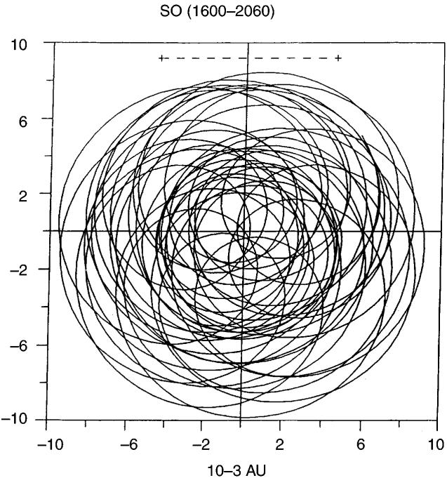
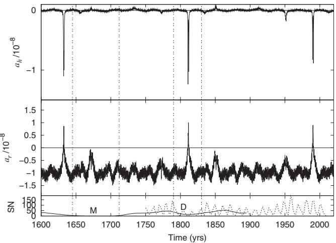
The geometry of the Sun’s motion around the Solar System barycentre is not a simple, smooth ellipse but a complex trajectory shaped by the gravitational pull of the giant planets, particularly Jupiter and Saturn. [180] This motion creates specific configurations of solar acceleration that have profound implications for solar activity. [203] Analysis of the normal component of solar acceleration, denoted as \(a_{h}\), reveals exceptional increases at specific epochs, which are explained by the inversion of angular momentum when the Sun’s orbit becomes retrograde. [203] This inversion aligns the angular momentum vector, L, towards the planetary acceleration direction, meaning that \(a_{h}\) represents the maximum projection of L in the solar acceleration direction, albeit in a contrary sense. [203] These changes are driven by orbital libration rather than an impulsive change in planetary acceleration, as planetary acceleration remains near the ecliptical plane. [203] However, these features are significant because they indicate that at times of angular momentum inversions, L is almost anti-parallel to the acceleration vector, with the angle between them oscillating between approximately 130 and 179 degrees. Crucially, these radial impulses never occurred before 1632 during the last millennium, even though similar planetary configurations did happen, demonstrating that these impulses arise only at epochs of orbital inversions and are responsible for particular phenomena. The periods of \(L_{z}\) inversion were characterized by a unique geometry of planetary acceleration with respect to the Sun-barycentre system, where the radial component of solar acceleration had an exceptional magnitude and the L vector was anti-parallel to acceleration. [203] However, further investigation is required to determine whether this relationship is causal or merely coincidental.
Solar barycentric dynamics, derived from a new solar-planetary ephemeris, reveal that orbital inversions are not strictly periodic in terms of the Jose-period but appear in irregular groups of three to nine events. [206] These retrograde motion intervals manifest with a bimillennial cycle, averaging approximately 2.2 kyr, yet within these broader periods, they do not occur regularly at the Jose-period. [206] For instance, some intervals of retrograde motion are separated by about 140 yr, such as between the years 2168 and 2308 or between -2458 and -2318. [206] Although the Jose-period beginning at -2458 is maintained, with another orbital inversion occurring at -2279, an intermediate lapse of retrograde motion takes place at the year -2318, which is 39.26 yr before the expected event of the year -2279. [206] Notably, before the retrograde interval of the year -2994, all orbital inversions inside each bimillennial cycle occur at the Jose-period. [206] The explanation for these shorter periods is straightforward: at each Jose-period, which is strongly related to the Uranus–Neptune synodic period of ~171 yr, a quasi-conjunction between Jupiter and the other giants tends to occur. [206] However, these quasi-alignments are not always able to produce a solar retrograde motion because of the ever-changing planetary positions and velocities at these particular events.
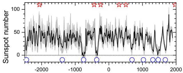
Analysis of the Sun’s barycentric dynamics reveals distinct radial impulses in solar velocity that align precisely with major periods of reduced solar activity. [203] This pattern demonstrates that radial impulses in the Sun’s velocity occurred at the beginning of the Maunder Minimum and Dalton Minimum. The alignment of these impulsive accelerations with historical grand minima confirms a phenomenological link between the barycentric motion of the giant planets and long-term solar cycle behavior. [70][203] Furthermore, the most recent impulsive event coincided with the maximum of cycle 22, preceding the current prolonged minimum of solar activity. Observational data show an apparent phase synchronization between sunspot numbers and the inclination of the orbital plane of the solar system barycenter, with correlation coefficients shifting from 0.76 to -0.52 after the radial impulse. [203]
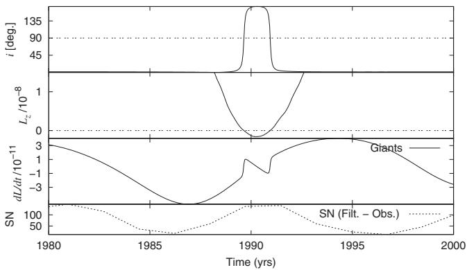
Analysis of the Sun’s barycentric dynamics reveals distinct impulsive events that correlate with major shifts in solar activity. [203] Specifically, a radial impulse in the Sun’s velocity occurred at the maximum of Solar Cycle 22, before the present extended minimum. This timing is significant because it coincides with a violation of the Gleissberg–Ohl rule involving cycles 22 and 23. [203] Although the nature of the current prolonged minimum remains unconfirmed, the accumulation of spotless days is comparable to that seen near the Dalton Minimum. [207] The radial component, which points toward or away from the barycentre, exhibits particularly dramatic changes during episodes of planetary quasi-alignments. [206] During these intervals, the Sun’s path undergoes orbital inversions, where the direction of its motion relative to the barycentre reverses. [203] The sudden changes in radial acceleration are so significant that they dominate the overall coplanar acceleration, which is the vector sum of the radial and tangential components. [203] These spikes in acceleration occur when the Sun fails to loop the barycentre, a phenomenon that happens when the barycentre lies outside the Sun’s orbital path. [203] This geometric configuration is a direct result of the specific alignments of the planets, which exert a combined gravitational force that pulls the Sun in a particular direction. [203] The magnitude of these acceleration spikes is much larger than the average values observed during other phases of the solar inertial motion. [203] The exceptional magnitude of the radial acceleration during retrograde intervals provides a clear signature of the planetary forcing on the Sun’s motion. [203] The separation of these two influences allows for a more precise understanding of the factors that drive solar variability. [124]
5.3 The Jose Cycle and Longer Beats
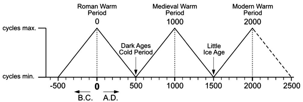
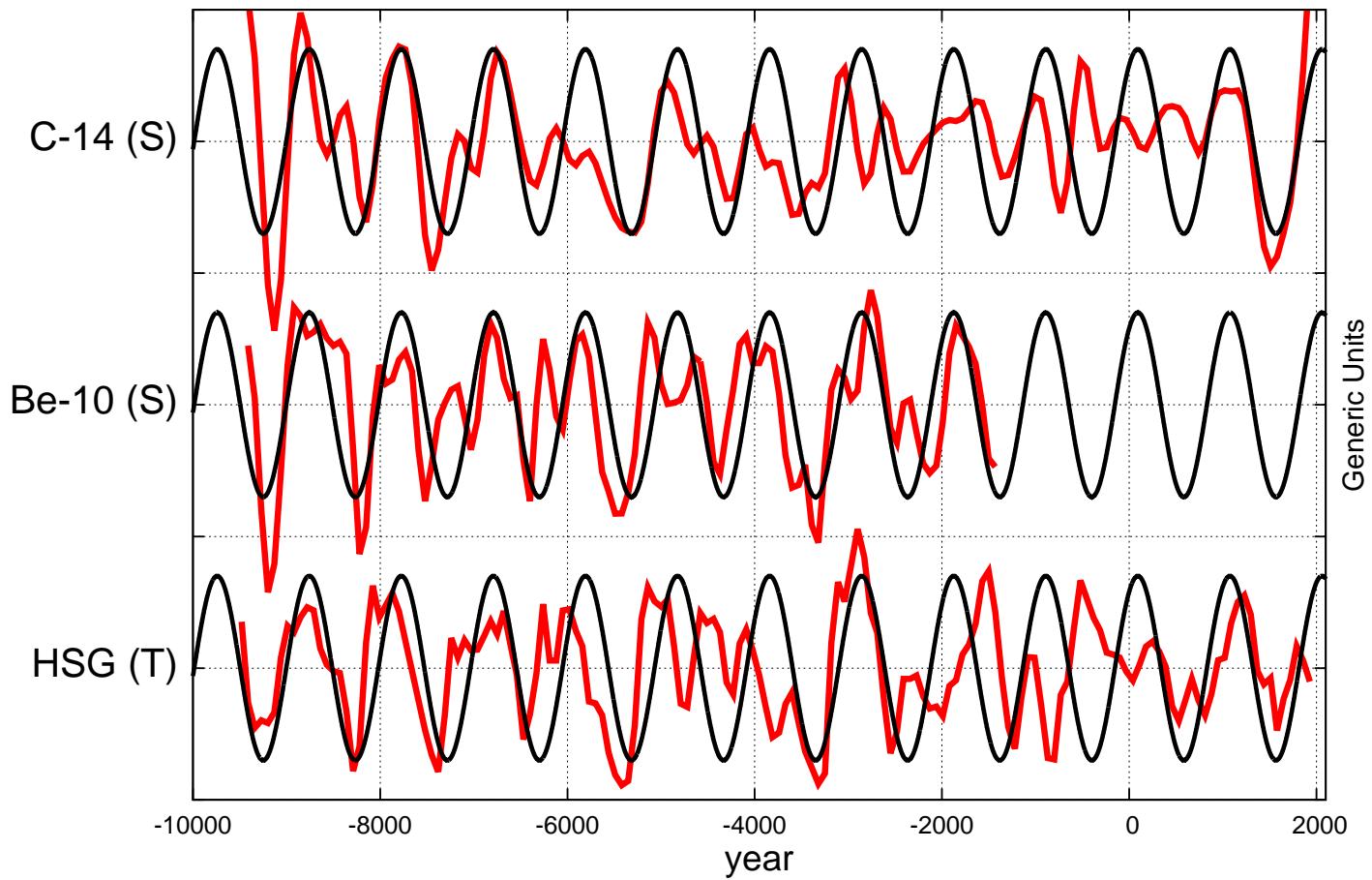
Power spectra of the sunspot record demonstrate that the 11-year Schwabe sunspot cycle is made up by three interfering cycles, which can be interpreted as due to the 9.93-year spring tidal cycle between Jupiter and Saturn, the 11.86-year Jupiter orbital tidal cycle, and a central oscillation of about 10.87 years that is almost, but not precisely, the average between the two tidal cycles and may emerge from the solar dynamo cycle as a collective synchronization harmonic. [209] This structure suggests that the 11-year Schwabe sunspot cycle consists of three periods linked to planetary orbital periods, including the Jupiter/Saturn spring period. Scafetta [11, 12] also noted that there are gravitational recurrence patterns of about 11.07-11.08 years due to the Mercury-Venus system and the Venus-Earth-Jupiter system, which correspond to the average solar cycle length. [209][127] Thus, numerous planetary tidal oscillations resonate around the 11-year Schwabe solar cycle, as postulated by Wolf. Taking these considerations into account, a simple solar model was developed by Scafetta involving just three harmonics, namely the two Jupiter/Saturn tidal cycles and a hypothetical solar dynamo cycle with a 10.87-year period. [209] This model reproduces a varying 11-year cycle that correlates approximately with the Schwabe sunspot cycle, and produces beats at about 61 years, 115 years, 130 years and 983 years, which are synchronous with major solar and climatic multidecadal, secular and millennial oscillations observed throughout the Holocene. [209] The model recovers the Roman Warm period, Dark Ages Cold Period, Medieval Warm Period, Little Ice Age, and Current Warm Period. [125] Instead of linking the periods of Sun’s long-term cycles to corresponding periods of planetary influences, another concept is pursued in which long-term cycles emerge as beat periods between the basic Hale/Schwabe cycle with the typical synodic periods of Jupiter with other Jovian planets. [127] The beat period of 193 years, as resulting from the 22.14-year Hale cycle and the 19.86-year synodic cycle of Jupiter and Saturn, has been noticed by several authors. [127] The aim is to corroborate how such beat periods actually emerge in a specific solar dynamo model, which had already demonstrated synchronization of the Schwabe cycle with the 11.07 years tidal period, based on the resonance of the intrinsic helicity oscillations of the current-driven m = 1 Tayler instability with the m = 2 tidal forcing. [127] The geometry of this solar orbit is essentially planar, with the Sun moving in the plane of the solar system, allowing for a clear separation into ordered and disordered orbital types. [70] This millennial-scale variability is further confirmed by analyses of the solar background magnetic field baseline, which reveal weak oscillations with a period of 2000 ± 95 years. [172] This millennial-scale oscillation is characterized by clustered occurrences of grand minima and maxima around its lows and highs, respectively, indicating a solar origin rather than purely climatic or geomagnetic variability. [113] The correspondence between the semi-Hallstatt cycle and the Eddy cycle indicates that the longer Hallstatt period is composed of two ~1000-year oscillations, corresponding to the Eddy cycle. This interpretation implies that the ~2200-year Hallstatt cycle may not be a fundamental solar mode, but rather an emergent property of two superimposed ~1000-year Eddy cycles. [36][8][113][15][111]
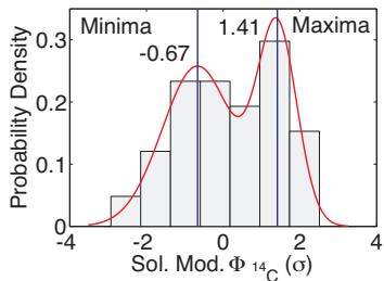
Analysis of the Holocene solar activity record reveals that the occurrence of grand minima is defined by stochastic or chaotic processes rather than long-term cyclic variations. Researchers examined possible quasi-periodicities in the rate of grand minima and maxima occurrence, finding only a weak, marginally significant quasi-periodicity of 2000–2400 years, a period well-known in \({}^{14}\)C data. [156][210][136][172] No other periodicities were observed in the occurrence rate of grand minima. [211] While a marginal hint for a periodicity of about 1200 years and its harmonics appeared in SN-S data for grand maxima, no periodic feature was found in the SN-L series. [211] This indicates that the 2400-year periodicity is related likely to the clustering of grand minima rather than to a long-term “modulation” of solar activity. [211] [124]
The statistical analysis of solar activity over the last millennia, derived from cosmogenic isotope records in natural terrestrial archives and historical sunspot data, reveals that the Sun spends the majority of its time at moderate activity levels, with approximately one-sixth of that duration characterized by a Grand minimum state and intermittent periods of Grand maximum activity. [210] While the occurrence of these extreme states is not the result of long-term cyclic variations but is instead defined by stochastic or chaotic processes, a distinct pattern emerges when examining the clustering of these events. [44] This long-term clustering is supported by the presence of a well-known period in radiocarbon data, as noted by Damon and Sonett and Vasiliev and Dergachev, which aligns with the marginally significant quasi-periodicity identified in the analysis. [211] The distinction between the clustering of grand minima and the occurrence of grand maxima is further clarified by the absence of periodic features in the grand maxima occurrence rate in the SN-L series, although a marginal hint for a periodicity of about 1200 years and its harmonics is found in SN-S data. [211] This evidence supports the conclusion that the 2400-year periodicity is related likely to the clustering of grand minima rather than to a long-term modulation of solar activity. [211]
5.4 Harmonic Analysis Yndestad and Abdussamatov
To isolate the long-term gravitational influences of the giant planets on the Sun’s motion, researchers must first strip away the rapid, short-period oscillations that dominate immediate orbital dynamics. [199] This separation is achieved through semi-analytical planetary motion theory, which relies on advanced mathematical techniques to average the Hamiltonian of the system. The Hori–Deprit method, a cornerstone of this approach, uses Lie transformations to systematically eliminate short-period perturbations from the equations of motion. By removing these high-frequency noise terms, the method allows for a much larger time step in the numerical integration of the equations of motion, making it feasible to model the slow, secular evolution of planetary orbits over centuries or millennia. [201] In recent implementations, such as those using the computer algebra system Piranha, the Hamiltonian of the four-planetary problem is expanded into a Poisson series in osculating elements of the second Poincare system. [201] The transformation between the original osculating elements and the new averaged elements is defined by change-variable functions derived from the second approximation of the Hori–Deprit method. [201]
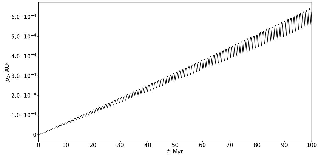
The algorithm proceeds by deriving second-order terms, \(H_{2}\) and \(T_{2}\), through the same procedural logic applied to first-order terms, maintaining consistency across the expansion hierarchy. [201] Crucially, the calculation of Poisson brackets, such as \(\{T_2, h_1 + \langle h_1 \rangle\}\), involves decomposing the expression into constituent parts like \(\{T_2, h_1\}\) and \(\{T_2, H_1\}\), with partial derivatives of \(T_2\) serving as change-variable functions computed by the \(chn\_n(2)\) script. This semi-analytical approach, constructed with computer algebra systems like Piranha to handle complex symbolic manipulations, contrasts sharply with purely numerical theories that yield only single trajectories and accumulate rounding errors. Instead, semi-analytical theories show insights into phase space properties and long-term stability, establishing a clearer view of the system’s dynamical behavior over extended periods. Applications to the Sun–Jupiter–Saturn–Uranus–Neptune system demonstrate the quasi-periodic nature of planetary motion up to 10 Gyr, with numerical integration of the averaged equations using Gragg–Bulirsch–Stoer and Everhart methods showing excellent agreement with numerical motion theories. [200][199][201] Specifically, simulations of the Sun–Jupiter–Saturn–Uranus–Neptune system over 100 Myr utilized the modified 15th-order Cowell–Störmer integrator and the symplectic Wisdom–Holman integrator, initialized with barycentric coordinates from the DE 430 ephemeris. [199] The results demonstrate that the osculating orbital elements derived from averaged equations maintain strong qualitative agreement with these direct numerical methods. [201]
The orbital evolution of the Sun–Jupiter–Saturn–Uranus–Neptune system on long time scales was studied using a Hamiltonian expansion into the Poisson series in elements of Poincaré second system, constructed up to third degree in the small parameter. [199] The estimation accuracy of this Hamiltonian expansion was evaluated by orbital elements of the Solar System’s giant planets, reaching about \(10^{-12}\). [199] The averaged Hamiltonian and the equations of motion in averaged Poincaré elements were constructed by the Hori-Deprit method up to third degree of the small parameter, with functions for the change of variables obtained in second approximation to transform between osculating and averaged orbital elements. [201] These constructed analytical equations of motion were applied to study the orbital evolution of the Solar System’s giant planets on long time scales with high precision, showing that the amplitudes and periods of the planetary motion are in good agreement with numerical theories. [199] The short-periodic perturbations of the orbital eccentricities and inclinations save small values over the entire interval of the integration. [200] Furthermore, the integration of the equations of motion with slightly different initial values of Uranus’ semi-major axis showed that the Lyapunov time for the orbits of giant planets is about 10–30 Myr. If the difference between the perturbing functions in the first and second approximations exceeds an amount obviously larger than the small parameter, this may testify to the presence of a resonance whose strength increases with this difference. [200]
The construction of semi-analytical theories for the orbital evolution of planetary systems, primarily focusing on the Sun–Jupiter–Saturn–Uranus–Neptune system and specific extrasolar systems such as HD 39194, HD 141399, and HD 160691, relies heavily on the Hori–Deprit averaging method. This framework utilizes Lie transformations to derive averaged equations of motion from the Hamiltonian expanded in powers of planetary masses, contrasting with purely numerical theories that provide only single trajectories and accumulate rounding errors. The process involves computer algebra systems, specifically Piranha, to handle complex symbolic manipulations for high-order approximations, expanding the Hamiltonian using Jacobi coordinates and the second system of Poincaré elements. [201] However, for extrasolar systems, the theory may be unacceptable near mean-motion resonances due to extreme growth in Hamiltonian terms. The real evolution of a system in this case, including the real presence of flips, can be studied only using numerical methods, confirming that symplectic integrators are essential for cases involving mean-motion resonances or orbital flips where analytical series diverge. Thus, the semi-analytical approach is best suited for secular evolution far from resonances, whereas numerical integration remains indispensable for capturing chaotic dynamics and resonance crossings. [213][200][199]
5.5 How Planetary Forcing Reaches Earth S Climate
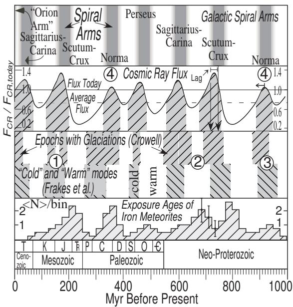
The statistical consistency between periodic spiral arm crossings, cosmic ray flux variations recorded in meteorites, and glaciation epochs over the past billion years suggests that these signals are not random phenomena. [213] By combining eight total measurements of HI data, the predicted spiral arm crossing period is estimated at 134.6 ± 22 Myr, while the period derived from Fe/Ni meteorites for cosmic ray flux variation is 143.6 ± 10 Myr. [213] These values align closely with the average observed recurrence period of glaciations on Earth, which stands at 145.5 ± 6.7 Myr. [213] A best-fit analysis comparing the actual prediction for the location of the spiral arms to the glaciations yields a periodicity of 143.65 Myr, suggesting that the phase of all three signals fits the predictions. [213] Specifically, the average mid-point of glaciations lags by 33.6 ± 20 Myr after the spiral arm crossing, consistent with the predicted lag of 31.6 ± 8 Myr. [213] Furthermore, the CR exposure ages of iron meteorites cluster around troughs in the glaciations, reinforcing the link between increased cosmic ray flux and reduced global temperature. This alignment suggests a non-random phenomenon for the appearance of glaciations with high statistical significance, indicating a potential connection between galactic structure and Earth’s climate history. Consequently, the data suggest that galactic environmental factors may play a significant role in modulating terrestrial climate cycles. [213] Thus, the SIM topology provides a potential mechanical basis for understanding how planetary forcing modulates insolation over long timescales, independent of internal solar dynamo processes.
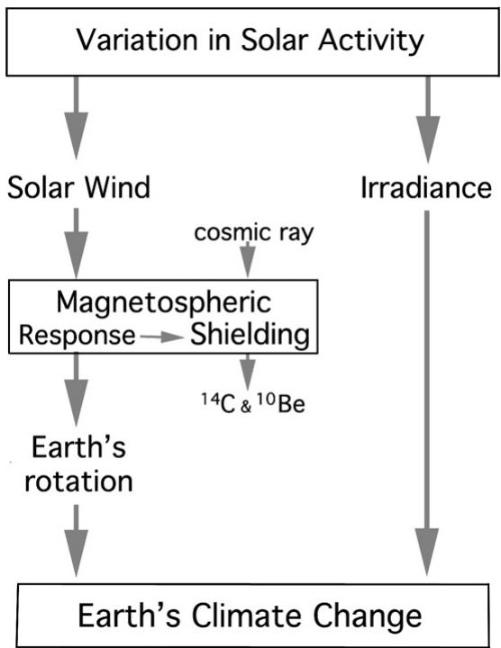
Solar wind variations interact with the Earth’s magnetosphere, a process that suggests changes in the planet’s rotation rate during solar minima. [214] This interaction alters the Earth’s total moment of inertia and atmospheric angular momentum, causing the interior rate of rotation to adjust as reflected in measured length-of-day variations. [215] These rotational shifts are associated with influences on ocean circulation and climate, particularly evident in the North Atlantic where speeding-up periods at grand solar minima may control main ocean surface circulation and Gulf Stream directional shifts. [214] The link between solar variability and terrestrial responses appears to go via the interaction of the Solar Wind with the Earth’s magnetosphere, which is consistent with observed rises and falls in sea level in the Indian Ocean. [187] Furthermore, the semi-annual component of changes in the Earth’s speed of rotation responds to changes in solar activity, supporting the idea that zonal wind circulation changes affect the speed of rotation of the planet. The Maunder Minimum time period, characterized by a lack of visible sunspots as noted by Eddy 1976, serves as a likely recent instance of reduced solar activity producing a noticeable effect on the climate system. [46] These findings challenge the notion that solar minima had negligible impact, suggesting that reduced solar activity significantly altered the thermal structure of the North Atlantic, thereby influencing global climate dynamics during these historical periods. [51]
The phasing of solar cycles indicates that a New Grand Solar Minimum may arrive by 2030–2040 — squarely inside the 2020–2053 window this book adopts — a prediction supported by convergent data from multiple independent analyses. [187] Dr. Theodor Landscheidt’s research at the Schroeter Institute for Research in Cycles of Solar Activity suggests a long period of cool climate with its coldest phase around 2030 — again within the 2020–2053 window — aligning closely with the author’s own calculations for the bottom of the next solar hibernation. [49] Peter Harris concludes there is a 94 percent probability of imminent global cooling. [49] Dr. S. Duhau and C. For the centuries preceding modern instrumentation, researchers have turned to cosmogenic radionuclides, specifically \({}^{10}\text{Be}\) and \({}^{14}\text{C}\), preserved in ice cores and tree rings, to reconstruct long-term trends in solar activity. [44] These isotopes are produced in the Earth’s atmosphere by nuclear reactions of cosmic ray particles with atmospheric nitrogen and oxygen, serving as a natural neutron monitor for cosmic radiation intensity. [56] However, it is crucial to recognize that these records do not measure total solar irradiance directly; instead, they reflect the modulation of galactic cosmic rays by the heliospheric magnetic field. Studies of Antarctic ice cores from the South Pole and Dome Fuji stations indicate that \({}^{10}\text{Be}\) variations provide a valuable proxy of solar activity, though complex production pathways and atmospheric transport processes impede quantitative interpretation. [67] Thus, while the planetary forcing mechanism provides the external trigger, the cosmogenic record confirms that the Sun’s magnetic response, not just its geometric position, is the variable that couples to Earth’s climate system.