8 There Is No Such Thing as Settled Science
Warming did occur, but the dominant driver was solar activity — not anthropogenic CO₂ — and the natural CO₂ budget plus low climate sensitivity make a CO₂-only attribution untenable.
8.1 Warming Happened but Who Did It
The twentieth century witnessed a pronounced warming trend, a fact that serves as the foundational premise for the dominant narrative attributing recent climate change primarily to anthropogenic carbon dioxide emissions. [244] In a pivotal study, Schurer et al. compared the expected signatures of high and low solar forcing against an ensemble of surface air temperature reconstructions for the past thousand years, carefully accounting for internal climate variability, volcanic eruptions, and uncertainties in both proxy data and model outputs. [292] Consequently, the mainstream interpretation holds that the warming observed in the Northern Hemisphere cannot be explained by solar cycles alone, setting the stage for a debate that centers on whether the current attribution models have adequately separated natural multi-decadal oscillations from anthropogenic signals or if they have inadvertently dismissed a more substantial solar contribution due to an underestimation of total solar irradiance variability and its potential amplification mechanisms. Their results demonstrate that while volcanic and greenhouse gas forcings contribute most to pre-twentieth-century climate variability, the contribution by solar forcing is modest. [292] Crucially, the study establishes that the 95% upper limit on the solar scaling factor rules out a solar contribution from the Maunder Minimum to present that is greater than about 0.15 K. This finding holds even when considering potential missing solar–ozone feedbacks, which would predominantly impact regional temperatures rather than enhancing the hemispheric mean response. [292] The authors conclude that for solar forcing to be a strong driver, the real-world climate sensitivity to it would have to be almost an order of magnitude smaller than in climate models, a scenario they consider highly unlikely. [292] Thus, the evidence shows that solar forcing is not a strong driver of large-scale Northern Hemispheric temperature variability over the past millennium, undermining the claim that solar activity alone accounts for the observed warming trend.
The global mean annual surface temperature increased 0.55°C from 1860 to 1990, a period coinciding with a steady rise in overall solar activity levels. [293] While standard climate models incorporating small total solar irradiance (TSI) changes of approximately 0.1% attribute recent warming primarily to anthropogenic greenhouse gases, this consensus view faces significant challenges from alternative reconstructions. [64] Temperature records derived from boreholes, such as the study by Huang et al., provide robust evidence for a 1.0–1.5 K difference between the Medieval Warm Period and the Little Ice Age, contradicting reconstructions that show minimal variation. [64] Consequently, some studies utilizing high solar variability estimates, which propose TSI changes of the order of 0.4%, argue that solar variability may have been the dominant cause of long-term warming since the 19th century. This perspective highlights the possibility that irradiance from the quiet Sun varies significantly in time, offering a natural explanation for the warming trend that does not rely solely on industrial CO₂ emissions. [64][31][1][46]
The unusual warming of the 20th century is mainly due to the coincidence of two highs in the 65-yr oscillation within the century, and an unusually high level of solar activity that reduced the mid-20th century cooling and increased the LTCW. [1] If we interpret the role of the interdecadal oscillation as a redistribution of heat from the lows to the highs of the oscillation, then this interpretation of MGW attribution assigns 10–20% of the 20th century temperature increase to GHGs, and 80–90% to solar activity. That 80–90% figure is the upper end of the solar-attribution estimates presented across this book — from the high-variability TSI reconstructions that make the Sun the dominant cause of the warming since the nineteenth century, up to this near-total attribution — and every one of them puts the Sun, not carbon dioxide, in the driver’s seat. The MSM is a period of 70 years with above average solar activity, representing the longest such period in the 320-yr sunspot record. [1] That the Modern Maximum coincides with the biggest period of warming in 600 years should not be considered as unrelated coincidence. [1] A test of this interpretation is about to take place. [62] Extrapolation of the forcings indicates we have entered, for the first time since 1900, a period when low solar activity coincides with a low in the 65-yr oscillation. [1]
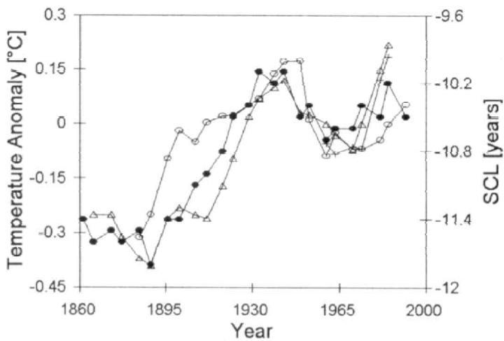
The official consensus within climate science, as articulated by Working Group I of the Intergovernmental Panel on Climate Change (IPCC), maintains that solar activity exerts only a limited influence on terrestrial climate dynamics. [8] However, this consensus overlooks abundant empirical evidence suggesting that the Sun has had a large influence on climate over the Holocene period, with temperature changes between periods of low and high solar activity reaching the order of 1–2 K. Such large variations are inconsistent with the consensus and herald a real and solid connection between solar activity and Earth’s climate, challenging the notion that solar effects are insignificant. [64]
The historical record provides a compelling counter-narrative to the idea that recent warming is an unprecedented anomaly driven solely by industrial emissions. [293] Specifically, the Wolf Minimum (c. Radiocarbon dating of pine tree rings, for instance, has identified a stationary climate oscillation of approximately 210 years that coincides with these grand minima, further supporting the link between solar variability and temperature shifts. [19] This historical precedent challenges the assumption that the twentieth-century warming trend is entirely novel. [94]
8.2 The Natural CO₂ Budget
The prevailing narrative of anthropogenic dominance often overlooks the fundamental sequence of events recorded in the deep past, where temperature changes clearly precede carbon dioxide fluctuations. [7] This temporal relationship is not a minor anomaly but a robust feature of the paleoclimate record; variations in CO₂ over the last 420 kyr broadly followed Antarctic temperature, typically by several centuries to a millennium. [7] The data establish that atmospheric CO₂ concentrations lag temperature increases by 800 ± 400 years during glacial terminations. For instance, at Termination III, a warming event that occurred over a 5000-yr period, the CO₂ increase occurred 800 ± 200 years after the Northern Hemisphere deglaciation. [295][7][296][297] The ice core data confirm that temperature leads CO₂, a fact that challenges the assumption that rising CO₂ is the sole or primary cause of recent warming. [297] The ocean acts as a vast reservoir, releasing gas as it warms, a process governed by Henry’s law. [8] The lag observed in the ice cores is consistent with this view, where temperature changes drive the carbon cycle, not the other way around. [295] Thus, the natural CO₂ budget, shaped by solar forcing and oceanic response, offers a coherent explanation for the observed CO₂ increases without requiring an exclusive attribution to human activity.
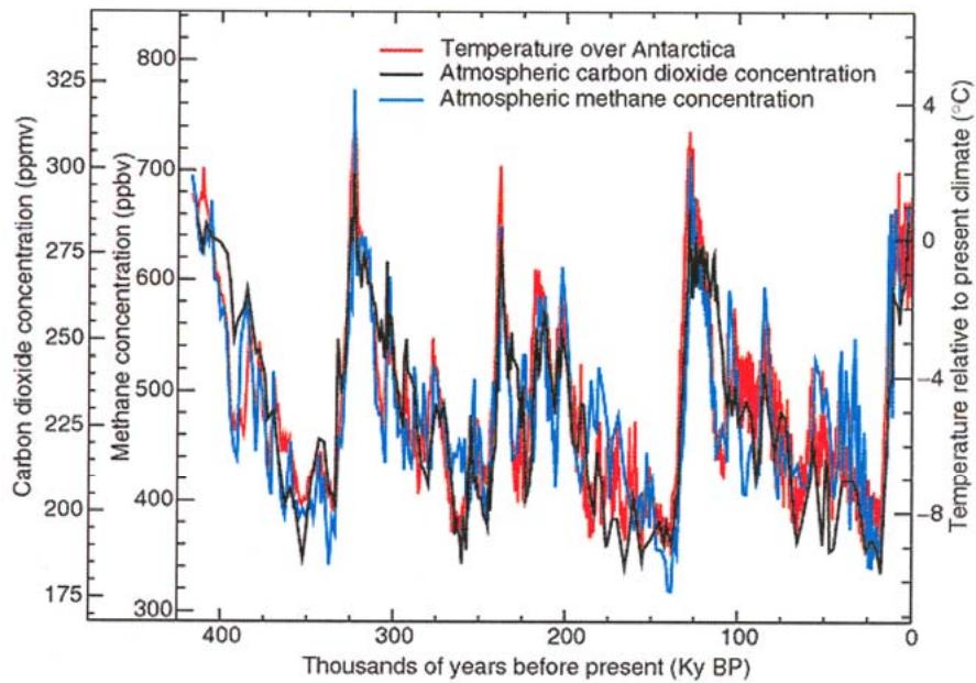
The oceans store approximately 50 times more carbon dioxide than the atmosphere, yet this vast reservoir is not static; its capacity to hold gas is strictly temperature dependent. [297] The historical record confirms this dynamic: during glacial terminations, temperature changes precede carbon dioxide shifts by 400 to 1,000 years, indicating that terrestrial temperature drives atmospheric carbon dioxide levels rather than the reverse. [298] Consequently, the observed increase in carbon dioxide since the Little Ice Age is consistent with natural ocean warming driven by solar heating, which reduces solubility and triggers outgassing. While carbon isotopic ratios indicate a contribution from fossil fuel burning, this accounts for only 1 to 5 percent of the total increase, suggesting that the dominant driver of rising carbon dioxide is the thermal response of the oceans to natural climate cycles, not anthropogenic emissions. [299]
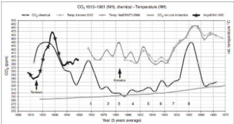
Modern observational studies suggest that atmospheric CO₂ changes lag global surface temperature changes by approximately 9 to 12 months. This temporal sequence is consistent with the mechanism where temperature controls the CO₂ level, as evidenced by MacRae who found that atmospheric CO₂ changes lag atmospheric temperature changes by about nine months. [1][296][52] Furthermore, Humlum et al. show that CO₂ increases consistently follow temperature increases by about 9 to 12 months, indicating that the correlation between cause and effect data proves there is no observable cause-effect relationship in the opposite direction. The lack of a statistically significant correlation between the rate of human carbon emissions and the rate of change of global surface temperature, even using time lags up to 20 years as found by Munshi, supports the view that temperature drives CO₂ rather than vice versa. [296] This aligns with the broader finding that CO₂ increases do not correlate with human CO₂ emissions but instead follow temperature increases, reinforcing the hypothesis that earth’s temperature is driving atmospheric carbon dioxide levels. [296] Thus, the observed lag and correlation patterns indicate that natural processes, particularly ocean outgassing driven by surface temperature, play a dominant role in atmospheric CO₂ variations. However, this foundation appears unstable when scrutinizing the historical measurement series. For instance, Charles Keeling’s acceptance of the French chemist Reiset’s data as the most accurate from the late 19th century ignored a critical methodological flaw: Reiset used sulphuric acid to dry the air before analysis. [10] Because sulphuric acid absorbs part of the CO₂, the results are too low by about 20 ppm, a fact known since 1848 and tested quantitatively by the Belgian chemist W. [10] Spring in 1883. Consequently, the correct average in the end of the 19th century was 312 ppm, not the 294 ppm that fit Keeling’s impression of pre-industrial levels. If the pre-industrial level was not 280 ppm, the argument that human CO₂ causes all the increase above that threshold loses its empirical grounding. [300] Beck’s reconstruction from chemical data further supports this, showing levels that reached 440 ppm in 1820 and again in 1945, contradicting the low proxy ice-core values that have dominated the discourse. These findings suggest that natural fluctuations may have played a more significant role than currently acknowledged. [300][10][7] Consequently, the attribution of recent CO₂ rises exclusively to anthropogenic sources remains open to debate. However, ice-core data from Siegenthaler and Joos indicate that natural CO₂ increased by 17 ppm, or 6 percent, before 1900, when human emissions totaled only 5 ppm, contradicting the assumption of constant natural variability. Furthermore, Beck’s reconstruction from chemical data shows the level reached 440 ppm in 1820 and again in 1945, suggesting that historical CO₂ levels were much higher than derived from ice cores alone. Jaworoski explains why ice-core data do not properly represent past atmospheric CO₂, concluding that nature produces 97 percent of atmospheric CO₂. [300] Analysis of ice core data through glacial and interglacial transitions consistently demonstrates an association between carbon dioxide and temperature, yet the climatic temperature always changed first, with carbon dioxide levels following after a measurable lag time of 400 to 1,000 years. [52] This sequence indicates that Earth’s temperature drives atmospheric carbon dioxide levels rather than the reverse, a mechanism explained by the vast storage capacity of the oceans, which hold far more carbon dioxide than the atmosphere. [16] Because carbon dioxide is soluble in water and its solubility decreases as water temperature increases, the gentle natural warming of the world’s oceans releases carbon dioxide into the atmosphere. [52] This physical process suggests that temperature-driven ocean outgassing is the main cause of the CO₂ increase since 1750, particularly as the oceans have warmed since the Little Ice Age. [296] The observed climate change is consistent with variations in albedo and associated ocean warming and cooling, supporting the view that this is merely a natural cycle evident in palaeoclimate data for most of the last 10,000 years. [299] At annual and 2-7 year time scales, the concentration of CO2 in the atmosphere is strongly driven by the ocean, and at longer time scales, greenhouse gas concentrations lag behind temperature. [299] Carbon isotopic ratios indicate that while there is a contribution from the burning of fossil fuels, it is of the order of 1-5 percent of the increase, implying that the warming of the oceans is a major contributor to the observed rise in CO2. [299] Furthermore, the Earth’s atmosphere is fairly stable and resilient; carbon dioxide levels during the Ordovician period were approximately 5,000 ppm, yet these high levels did not throw the world into runaway global warming. If exceptionally high carbon dioxide levels did not cause runaway global warming in the past, it is reasonable to question why minimal levels of 387 ppm would do so in the future, reinforcing the conclusion that the available evidence indicates climate change is predominantly natural and occurs mostly in response to variations in solar heating of the oceans. Consequently, the attribution of recent warming primarily to anthropogenic emissions appears to be an oversimplification of a complex, naturally driven system. [52][299][298][297][301][300]
8.3 The Surface Temperature Record Under a Magnifying Glass
The integrity of the global surface temperature record remains a focal point of contention, particularly regarding the influence of urbanization on land-based measurements. [101] This shift is particularly acute in regions like China, where rapid acceleration in urbanization has transformed most formerly rural stations into urbanized sites, suggesting that urbanization bias is a persistent problem for many station records. [148] Consequently, the reliance on homogenization algorithms to smooth through excess warming in cities may inadvertently smear warmer urban temperatures over large areas, potentially inflating the Global Surface Air Temperature (GSAT) estimates used in recent assessments.
The standard defense of global temperature datasets relies on statistical homogenization techniques, such as the Menne & Williams algorithm, which are designed to remove non-climatic biases from raw station records. [148] Proponents argue that these automated methods substantially reduce urbanization bias, thereby rendering the combined urban and rural data representative of true hemispheric trends. [101] However, this confidence is challenged by evidence suggesting that the algorithm performs poorly when a substantial fraction of neighboring stations share similar non-climatic biases. In such scenarios, the method can lead to “urban blending,” a process where the urbanization bias of heavily urbanized stations is not removed but rather averaged with neighbors. [148] Consequently, if rural stations are few, they may have artificial urbanization bias introduced into their records, effectively aliasing the urban signal onto rural trends. Critics dispute homogenization methodologies, arguing they may inadvertently cause ‘urban blending’ that aliases urban bias onto rural stations. This implies that the homogenized Global Historical Climatology Network may retain significant systematic errors, particularly in regions where siting biases are widespread, undermining the assumption that statistical adjustments fully correct for the urban heat island effect. [148][51][101]
The integrity of the terrestrial temperature record since 1900 faces scrutiny from urban heat-island effects, which may distort the apparent warming trend. [8] Analysis of 5x5 degree grid boxes by Jones and Moberg reveals that statistically significant warming trends are present in only 10–20% of available boxes, with most land-area warming concentrated near large cities and urban centers rather than being uniformly distributed. [303] This spatial correlation suggests that urbanization and land-use change, rather than greenhouse gases, drive the most pronounced local increases. [303] Further evidence indicates that standard adjustments for these non-climatic factors are insufficient. [8] Ross McKitrick and Patrick Michaels demonstrated a strong correlation between urbanization indicators and “urban adjusted” temperatures, concluding that fully correcting the surface temperature data for such extraneous factors reduces the estimated 1980–2002 global average temperature trend over land by about half. [8] Similarly, Jos de Laat and Ahilleas Maurellis found a statistically significant correlation between the spatial pattern of warming and industrial development, adding a large upward bias to the measured global warming trend. [8] The experience at the Urbana, Illinois site underscores this challenge, where a gradual warming of 0.9°C occurred as the university campus grew around the station from 1900 to 1983, followed by immediate cooling upon relocation to a rural setting. [8] These findings suggest that inadequate urban heat-island adjustments could account for up to half of apparent terrestrial warming since 1900. Consequently, the magnitude of anthropogenic warming may be substantially overstated if these localized biases are not fully accounted for. [303][8][304]
The integrity of the surface temperature record hinges on whether urbanization has introduced a measurable warming bias, a question that remains contentious despite widespread assertions to the contrary. [148] While some analyses suggest minimal impact, empirical comparisons between urban and rural stations reveal significant temperature differences that contradict claims of no statistically significant urbanization impact. This discrepancy is not merely theoretical; it manifests in concrete data from diverse global locations. [8][148][101] For instance, Ren et al. noted that annual urbanization-induced warming at Beijing and Wuhan stations accounted for about 65–80% of the overall warming in 1961–2000, demonstrating that local anthropogenic effects can dominate regional trends. [148] Similar nocturnal warming and daytime cooling patterns were observed in California’s Central Valley by Christy et al., where increased irrigation suppressed daytime temperatures via evaporative cooling while warming nights through increased heat capacity. [8] These findings, echoed in studies across China, Europe, and even remote villages like Barrow, Alaska, confirm that urban heat-island effects are pervasive and often greatest at night and in higher latitudes during winter. [8] Consequently, the assertion that current surface air temperature records are free from urbanization-induced bias is undermined by numerous studies showing significant warming in urbanized areas, necessitating careful scrutiny of homogenization procedures that may inadvertently retain these artificial signals rather than removing them.
The construction of rural-only station composites serves as a critical methodological check, designed to avoid the potential artifacts introduced by homogenization procedures and thereby provide an alternative estimate of temperature trends. This approach is particularly relevant in regions with a high density of rural stations, where the distinction between raw and adjusted data can significantly influence the perceived magnitude of warming. [101][148] The underlying premise is that raw rural records may offer a more authentic representation of broader climatic shifts, especially when compared to homogenized datasets that incorporate both urban and rural observations. [101] This distinction is vital because the homogenization process, while intended to correct for non-climatic biases, can sometimes introduce its own set of uncertainties. [148] Consequently, the resulting rural-only composites suggest that the temperature trends derived from these unadjusted records might differ from those obtained using standard global datasets. This divergence highlights the importance of scrutinizing the data sources and processing methods used in climate studies, as the choice between raw rural data and homogenized global records can lead to different interpretations of historical temperature changes. [101]
The integrity of the surface temperature record, particularly in regions undergoing rapid development, remains a subject of rigorous scrutiny. [148] In China, for instance, the times of observation since 1953 appear to have been well regulated, yet this level of consistency does not seem to have been the case for earlier records. [148] While it is plausible that some of the net adjustments applied by Menne & Williams are a result of correcting for time of observation bias, the evidence suggests that such biases are quite modest for the Chinese network. [148] Tang & Ren attempted to partially account for time of observation bias by using a combination of maximum and minimum temperature records, yet their reconstruction was quite similar to the gridded mean average when using the non-homogenized dataset. [148] This similarity suggests that the net biases from changes in time of observation are quite modest for the Chinese network. [148] Still, this does not rule out the possibility that the relatively large pre-1950s Menne & Williams adjustments may be correctly removing some other non-climatic biases, such as those introduced by station moves. On the other hand, when the number of fully rural stations in an area is low, as was the case pre-1951, homogenization algorithms such as the Easterling & Peterson 1995 algorithm used by Li et al. will lead to urban blending. [148] This process means that the urbanization bias will tend to be distributed amongst all stations, both urban and rural, to generate a uniform “homogenous” blend. [148] Indeed, the magnitude of the adjustments for the pre-1951 period is actually greatest for the fully rural subset, and the homogenization algorithm reduces the warmth of the mid-20th century warm period, effectively introducing a warming trend into the fully rural subset. This pattern is consistent with urban blending. [148] If the homogenization algorithm has indeed introduced urban blending, then this would have reduced the reliability of the station records, rather than improved it. [148] Consequently, homogenization adjustments in Chinese records pre-1951 are greatest for rural subsets, potentially introducing artificial warming trends via urban blending. This mechanism explains why Li et al. failed to identify much urbanization bias in their analysis, as the algorithm effectively masks the very signal it seeks to correct. [148] The implication is that the rural-only composites, often cited as cleaner proxies for natural variability, may themselves be contaminated by the statistical artifacts of homogenization. [148] When urban blending occurs, the distinction between rural and urban stations blurs, and the resulting composite inherits the urban heat island bias. [148] This does not negate the warming itself, but it does complicate the attribution of that warming to specific drivers. [305] The lesson from the Chinese records is that homogenization is not a neutral process; it can actively reshape the temperature trend, especially in periods with sparse rural coverage. [148]
8.4 TSI vs CO₂ the Connolly Soon Attribution
Central to this alternative view is the realization that the deep ocean carbon stores are so vast that carbon sinks can be considered unlimited in terms of anthropogenic emissions, a fact supported by large \(\delta^{13}C\) excursions associated with the formation of large igneous provinces that formed over tens of thousands of years. [1] By recognizing that constant current emissions lead to a new equilibrium at 240 ppm above the present value, we see that the system is self-regulating through deep ocean carbon stores. [1] Thus, the focus shifts from panic over emissions to understanding the solar and natural cycle drivers that truly govern our climate, setting the stage for a more accurate assessment of future warming trends and the potential return of cooler conditions.
The historical temperature record for Greenland provides a critical test of anthropogenic forcing, as fluctuations over the past 500 years predate large CO₂ emissions and cannot be caused by them. Merged data from 1784 to 2005 reveal that the warmest period occurred in the pre-World War II era, specifically the 1930s and 1940s, before the massive global industrialization of the last 70 years and the emission of most greenhouse gases. [49][306][7][2][307] Furthermore, southern Greenland experienced a cooling of 1.29°C between 1958 and 2001, adding to the ice sheet’s mass balance. These findings demonstrate that natural variability, rather than industrial emissions, drove these temperature shifts, ruling out CO₂ as the primary driver for the observed changes in the Greenland record. [8]
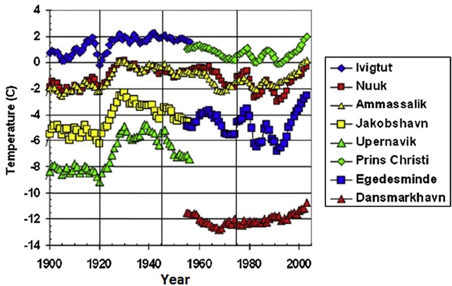
The mid-century cooling trend from 1945 to 1977, which occurred despite a significant post-1945 increase in CO₂ emissions, demonstrates that rising greenhouse gases were not the sole determinant of surface temperatures during that era. This period of cooling, juxtaposed against increasing anthropogenic forcing, challenges the assumption that CO₂ dominates short-term climate variability. [8] Instead, it suggests that natural factors, such as solar activity and internal climatic oscillations, played a substantial role in modulating global temperatures. [1] The coincidence of this cooling with specific phases of the ~65-year oscillation and solar cycles indicates that these natural drivers can counteract greenhouse warming on decadal timescales. [1] Consequently, the temperature record from 1945 to 1977 provides critical evidence that the climate system’s response to forcing is more complex than simple CO₂-driven warming, highlighting the need to account for natural variability in attribution studies.
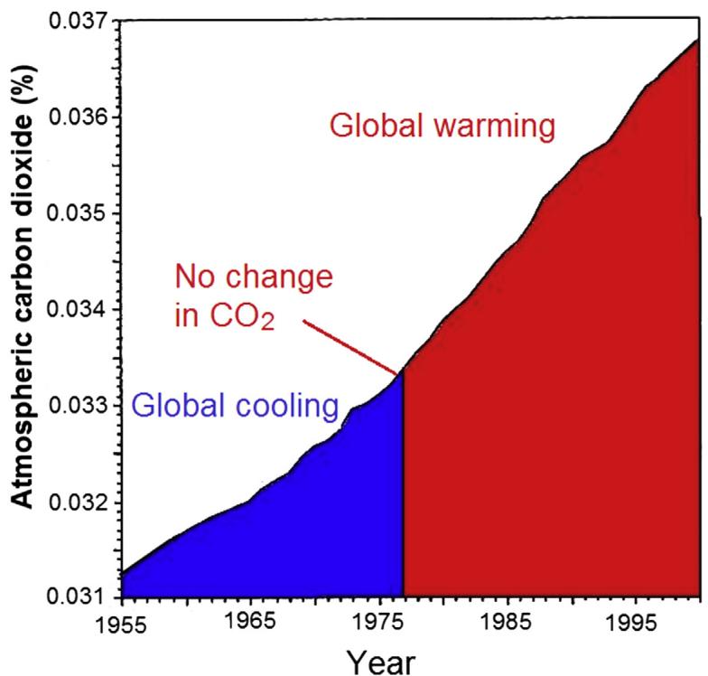
The attribution debate hinges on whether solar variability or greenhouse gases drove the twentieth-century warming. [244] While standard models assign a minor role to the Sun, alternative analyses suggest a much larger solar contribution. [243]
The discrepancy between predicted and observed temperature changes suggests that the IPCC’s central value for doubling sensitivity, (S = 3.0 C), is far too large. [308]
The attribution debate hinges on which forcing best explains the observed warming. [1] The unusual warming of the 20th century is mainly due to the coincidence of two highs in the 65-yr oscillation and an unusually high level of solar activity that reduced mid-century cooling. [1] If this interpretation holds, the overwhelming share of the modern temperature increase belongs to the Sun rather than to greenhouse gases — the quantitative split was set out at the opening of this chapter. [1] This apparent success demonstrates that the models rely on several adjustable parameters, chosen specifically to produce agreement with the observed global average surface temperature, rather than robust physical constraints. The uncertainty in climate sensitivity, defined as the temperature increase produced by a doubling of greenhouse gas forcing, is a factor of three or larger, yet the IPCC presents a narrow range of 1.5 to 4.5 degrees Celsius. [309][7][1][308][46] Furthermore, the forcing effects from aerosols are highly uncertain, by at least 200% for the cloud-reflective effect, which is used in the construction of the attribution graphs. By tweaking these parameters, the models can match the “predicted” warming, but this fine-tuning obscures the fact that the projections fail to catch the actual temperature variations and cyclicities of the past 100 years. [7] The reliance on such adjustable inputs suggests that the attribution of warming to anthropogenic causes is not unequivocally tied to physical evidence, but rather to model assumptions that can be scaled to fit the data. [1]
The synthesis of solar attribution rests on the deep-time consistency between solar modulation and terrestrial climate, a relationship that extends far beyond the instrumental era. [64] John Eddy’s early observations of the correlation between solar activity and European climate over the previous millennium further anchor this long-term trend. [64] This alignment suggests that the Sun’s influence on climate is not a short-term anomaly but a persistent driver operating on decadal to millennial timescales. [64] It challenges the notion that recent warming can be attributed solely to anthropogenic factors, instead pointing to a natural cycle that has governed Earth’s climate for centuries. [1]
8.5 Natural Cycles as Confounders Scafetta AMO PDO
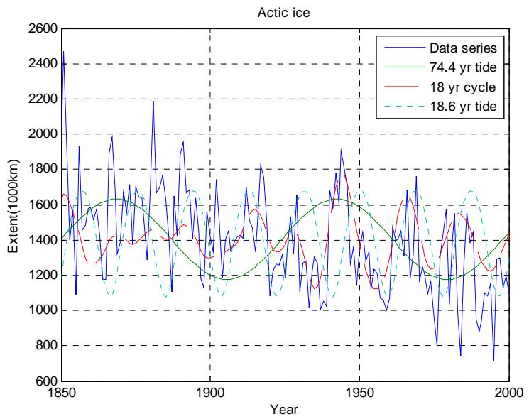
A compelling example of such deterministic forcing is found in the Barents Sea, where long-term temperature records reveal clear periodicities linked to lunar mechanics. [310] If similar cycles operate globally, they could account for a substantial portion of the observed warming, thereby undermining the assumption that CO₂ is the primary driver. [305] Wavelet analysis of Arctic ice extent data reveals dominant cycles of approximately 18 and 74 years, mirroring patterns found in polar motion and North Atlantic water records. [311] Specifically, this 74-year cycle associated with polar position variations correlates with cold Arctic water outflow, indicating that lunar gravity modulates the release of cold water from the Arctic Ocean into the Greenland Sea. The phase delay between the polar-position cycle and the Greenland ice extent is estimated at about 18.5 years, representing a significant lag in the circulation of Arctic water. [312][311] This delay supports the view that the Arctic system does not respond instantaneously to forcing but rather integrates signals over decades. [90]
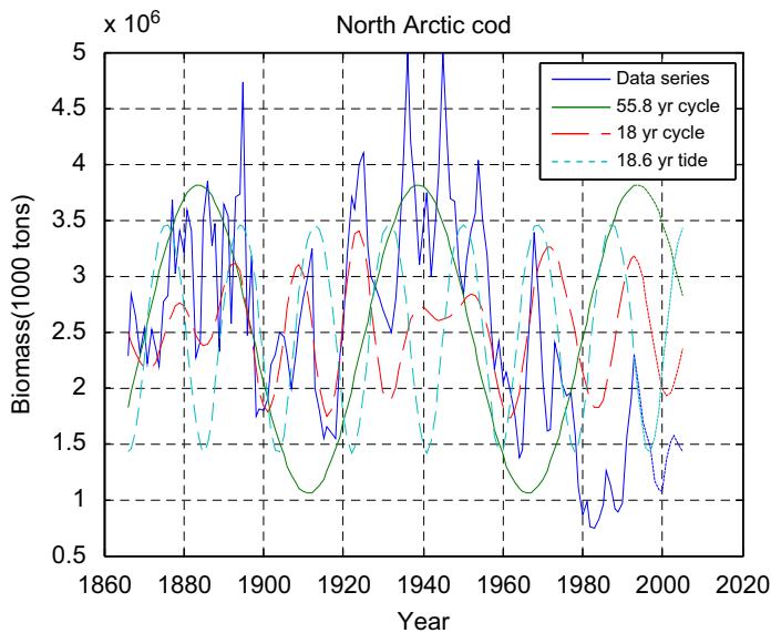
The systems dynamics of North arctic cod operate as a non-linear, time-varying process dependent on ecology and landings systems, revealing a dynamic process closely correlated to temperature cycles of 3 × 18.6 = 55.8 years, 18.6 years, and 18.6 / 3 = 6.2 years. [313] These temperature cycles are related to changes in the earth nutation and thus expected to be deterministic, with the 6.2 year cycle influencing cod recruitment, growth rate, and landings, while the 18.6 and 55.8 year cycles influence growth rate and maximum biomass. [313] This deterministic structure suggests that a control strategy can manage the dynamics introduced by these temperature cycles, opening the door for simplified dynamic modelling and forecasting of future biomass. [313] Consequently, deterministic cycles allow prediction of long-term temperature fluctuations using Multi-Layer Feedforward Networks, which appears to support the view that Arctic temperature and biomass fluctuations follow predictable patterns rather than random noise. The climatological baseline, such as the Roemmich-Gilson climatology, treats the ocean as an Eulerian field, averaging measurements at fixed geographic locations over time. [314] However, ocean temperature is fundamentally a Lagrangian property, characteristic of specific water masses that move, mix, and transform as they are advected by currents. A water mass at 30° N, 150° W in January 2005 and another at the same coordinates in January 2018 are not the same physical entity; they possess different histories, source regions, and thermodynamic states. [314] Averaging their temperatures produces a statistical artifact rather than a meaningful physical baseline. [314] This Eulerian-Lagrangian mismatch is compounded by the temporal arbitrariness of the chosen averaging period. [314] The baseline is derived from smoothing measurements over the 2004–2018 period, a 15-year window that is physically arbitrary. [314] Major ocean processes, including mesoscale eddies, seasonal convection cycles, the El Niño-Southern Oscillation, the Pacific Decadal Oscillation, and Atlantic Multidecadal Variability, operate on timescales incommensurate with this averaging period. [314] Consequently, the resulting climatology reflects the specific dynamical state of the ocean during 2004–2018, including whatever phase each oscillatory process occupied, rather than any physically meaningful equilibrium state. Furthermore, changing float density and persistent spatial sampling gaps in polar domains introduce systematic biases, particularly when constructing climatological reference states.
The reliability of the Earth Energy Imbalance (EEI) assessment is called into question by the physical validity of the underlying Argo-float-based estimates of global Ocean Heat Content (OHC). [314] Rather than canceling out globally, these displacements are governed by local, non-stationary processes such as eddies, fronts, and turbulent shear, which introduce incoherent regional errors into Eulerian gridded fields. [314] When these errors accumulate, they create a time-dependent methodological bias in OHC trends, particularly when combined with interannual circulation variability like ENSO or PDO shifts. [314] A rough scaling suggests this effect could shift global EEI estimates by on the order of 0.02–0.1 W m\(^{-2}\), a range comparable to or exceeding some published ensemble spreads that do not account for this foundational data-assignment flaw. [314] Furthermore, similar artifacts arise from how the reference climatology is constructed, where temperature profiles measured at different times during each month are pooled together and statistically fitted. Consequently, the confidence in EEI trends derived from these datasets is undermined by these unresolved methodological uncertainties. This uncertainty is not merely theoretical; it is embedded in the very metrics used to quantify the planet’s energy state. [314] When these errors are synthesized, the resulting uncertainty is far larger than officially reported. [314] Consequently, the apparent energy accumulation driving the warming narrative may be an artifact of interpolation in unsampled volumes and framework discrepancies rather than a robust physical signal.