3 Solar Science Foundations
The instrumented solar record — sunspot counts, magnetic indices, F10.7, TSI — is the toolbox every later chapter draws on.
3.1 From Galileo to the Photoheliograph
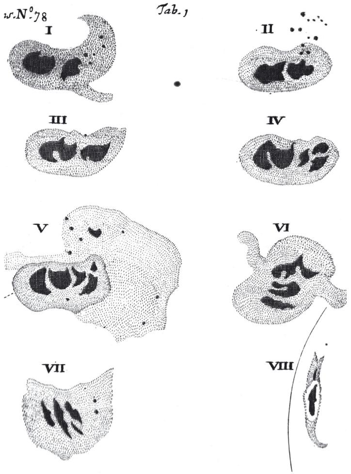
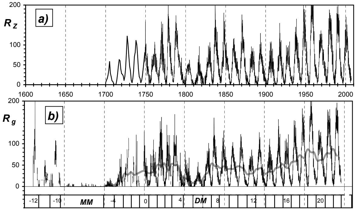
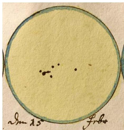
The history of solar observation begins not with the naked eye, but with the lens. [44] Almost as soon as telescopes were turned toward the Sun, observers noticed dark blemishes — sunspots — drifting across its face. By the late seventeenth century, astronomers like Cassini and Flamsteed were tracking the frequency of these spots with increasing regularity. [109] Cassini noted that spots were more frequent in 1676 than in the twenty years preceding, while Flamsteed lamented their rarity in the years following. [109] The sunspot number, a key metric in solar physics, traces its lineage back to these early observations. [62] The legacy of 1610 is thus not just a historical footnote, but the starting point of the solar record that underpins our current understanding of solar variability. [44] This method allowed for relatively good solar images and remained in use until the late 18th century. [44] The first known observation of a sunspot using a camera obscura — a darkened chamber that projects an image of the Sun through a small aperture onto a screen — was done by Kepler in May 1607, who erroneously ascribed the spot on the sun to a transit of Mercury. [44] Although such observations were sparse and related to other phenomena, such as solar eclipses or transits of planets, there were also regular solar observations by camera obscura. [44] For example, about 300 pages of logs of solar observations made in the cathedral of San Petronio in Bologna from 1655–1736 were published by Eustachio Manfredi in 1736. [44] These records demonstrate that observations and drawings made using camera obscura can be regarded as instrumental observations, despite predating widespread telescope use. This classification is crucial because it establishes a continuous record of solar activity that bridges the gap between naked-eye sightings and the systematic telescopic surveys that followed. [110][111][109][112]
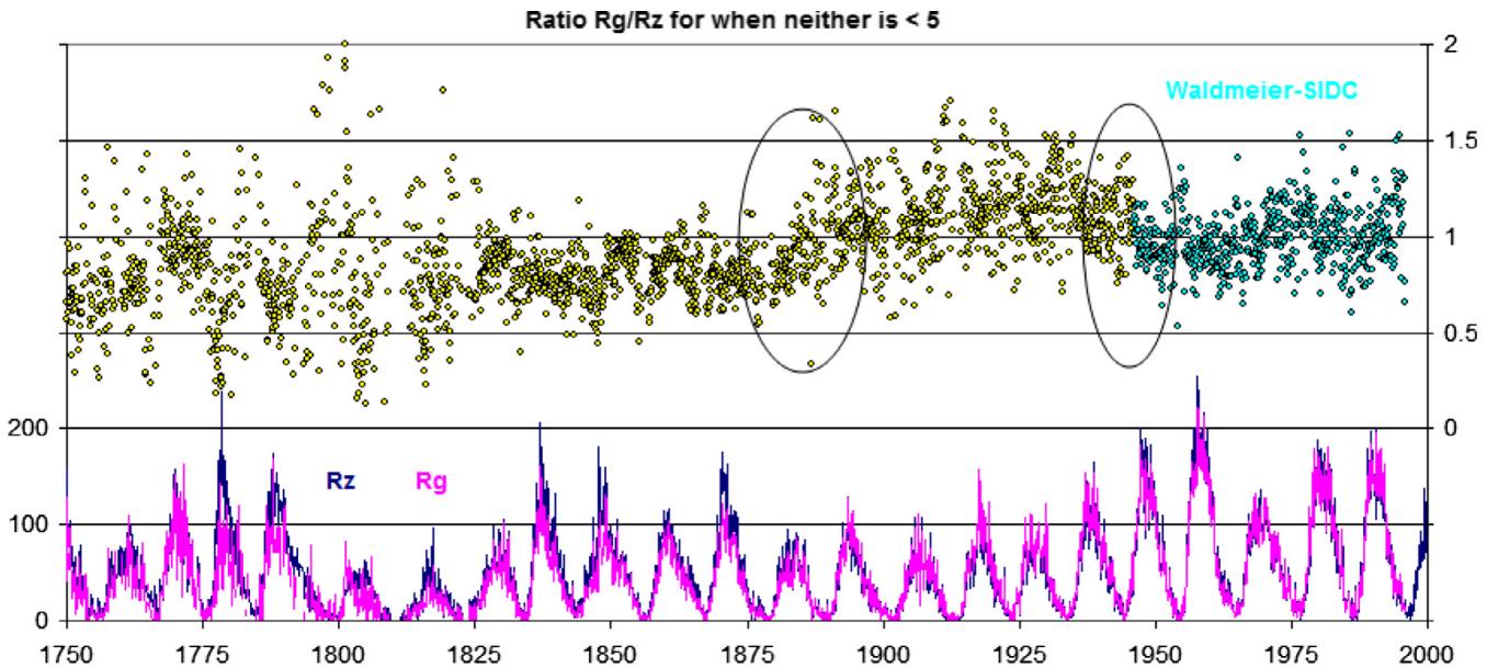
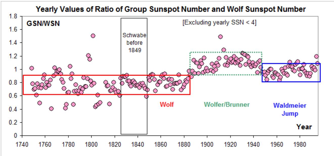
The sunspot number stands as the most common and longest available index of solar activity, serving as a synthetic index useful for the quantitative representation of overall solar activity outside the grand minimum. [44] However, this series has big uncertainties before 1900, and fragmentary non-instrumental observations of the sun before 1610, while giving a possible hint of relative changes in solar activity, cannot be interpreted in a quantitative manner. Daily records of sunspot observations have formed an essential basis for evaluating long-term solar activity since 1610, a data series often considered one of the longest ongoing scientific experiments in modern science. [110] After the initial modern compilation of the comprehensive data set of sunspot group number in Hoyt & Schatten (1998a, 1998b), recent studies have continuously recalibrated and improved these data series to revise the overall long-term trends. [110] Investigations of the original observational records have formed the basis for these analyses, offering a ground truth for further recalibrations using sophisticated methods. [110] The standard sunspot number index is available from 1610 AD onward, though data quality degrades significantly in earlier periods. Consequently, interpretations of solar activity prior to the twentieth century should be treated with caution due to these inherent observational limitations. [113][110][111][114][115][116] This adjustment, attributed to Max Waldmeier, significantly altered the Relative Sunspot Number, creating a discontinuity in the ratio between the Group Sunspot Number and the Standard Sunspot Number around 1945. [117] However, systematic searches of historical drawings from the Greenwich Photoheliographic Programme suggest that the earlier observer, Wolfer, did not apply this weighting scheme, as no such spots were found in the records for which weighting was allegedly applied at Zürich. This finding is consistent with the absence of any mention of a weighting scheme in Wolf’s and Wolfer’s meticulous yearly reports in the Mittheilungen über Sonnenflecken series. [62] Consequently, the apparent continuity of the record masks a fundamental shift in observation protocols, where the Locarno Station, serving as the modern reference site, continues to apply Waldmeier’s weighting, thereby carrying the effect fully into the current sunspot number maintained by SIDC in Brussels. Thus, the recovery of lost notebooks is not an antiquarian exercise but a necessary step to establish a reliable baseline for comparing modern satellite-era measurements with pre-telescopic reconstructions.
3.2 Cycle Metrics Schwabe Hale Butterfly
This variability is anchored by the Schwabe cycle, an approximately 11-year period of solar activity that serves as the primary heartbeat of the solar dynamo. [119] Space-borne measurements of total solar irradiance (TSI) and spectral solar irradiance (SSI) clearly establish this 11-year cycle, showing that while the overall energy output varies by only about 0.1%, the ultraviolet spectrum fluctuates by several percent, particularly in the 200–250 nm range. This modulation is not merely a surface phenomenon but is deeply tied to the Sun’s magnetic structure. [120][121][122][123] This longer magnetic cycle is evident in the modulation of galactic cosmic rays, which exhibit a 22-year pattern influenced by the tilt of the heliospheric neutral current sheet — the vast, rippled surface winding through interplanetary space that separates the two magnetic polarities of the Sun’s field — and the drift of charged particles through the interplanetary magnetic field. [122] The connection between magnetic activity and irradiance is further confirmed by observations of the Ca II H and K emission lines, whose cores are heated by magnetic processes in the chromosphere, the thin layer of the Sun’s atmosphere just above its visible surface. [120] These lines serve as a quantitative proxy for stellar magnetic activity, revealing that more active stars possess more vigorous cycles, implying that the younger Sun likely experienced stronger irradiance variability than it does today. [120] Together, these cycles create a complex, asymmetric environment that modulates the flow of cosmic rays and shapes the space weather experienced by Earth. The ~11 yr cycle itself was discovered by Heinrich Schwabe in 1844 through tracking the variation in the sunspot number. [44] This ~11 yr cycle is considered a fundamental feature of solar activity originating from the solar dynamo process. It is currently believed that these quasi-periodic changes in solar irradiance and sunspot number, known as the Schwabe cycle, are the result of solar differential rotation as modeled in hydromagnetic solar dynamo models. [124][125][126][127][128] Half a century later, E. W. Maunder identified the butterfly diagram, a pattern progressing from ~30° latitude to the equator over the ~11 yr period. [129] Later, G. E. Hale demonstrated that sunspots were sites of intense magnetism protruding through the Sun’s photosphere and that the polarities of the butterfly’s wings alternated in sign with a period of about 22 yr. [126] The variability of solar cycle amplitudes from decadal to millennial timescales can be understood as the natural behaviour of the solar dynamo itself — a weakly driven, noisy oscillator. [124] No intrinsic periodicities apart from the 11-year cycle are required to understand this variability, although the possible existence of such periodicities cannot be strictly excluded. [124]
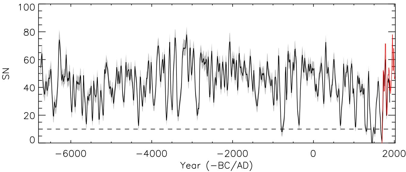
Sunspot number remains the main parameter used to track this periodicity, but the count is only the surface signature of a deeper magnetic rhythm. [130] The real physical period of the solar activity cycle is therefore not 11, but 22 years, as the sign of the toroidal magnetic field in any given cycle is opposite to that in the preceding cycle. [131] This alternation is reflected in Hale’s polarity law, which notes that the leading polarity in each hemisphere changes from one sunspot cycle to the next. [130] Consequently, the 22-year Hale cycle represents the full magnetic polarity cycle, where sunspot polarities alternate in sign each 11-year cycle. This magnetic reversal implies that the large-scale organization of the magnetic field in the interior is mostly toroidal in orientation — wrapped around the Sun’s rotation axis in belts, rather than running pole to pole — and oppositely directed on either side of the equator, a pattern that active regions adhere to approximately 92–95% of the time. [132][126][133][134][135][136]
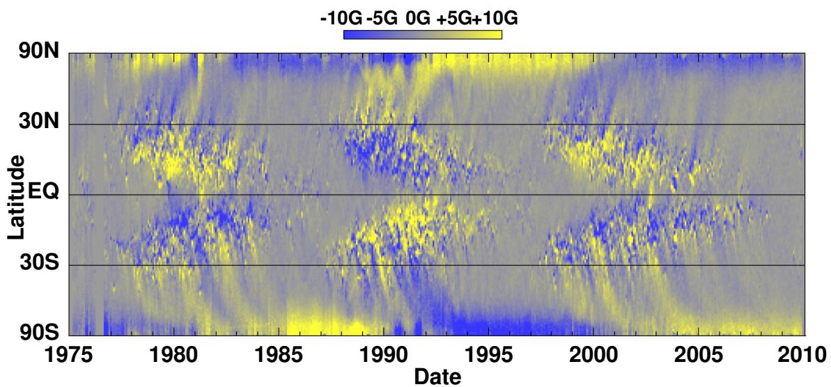
The solar cycle is not merely a fluctuation in spot counts but a complex magnetic phenomenon with distinct spatial and temporal signatures. [130] The butterfly diagram shows sunspot emergence progressing from approximately 30 degrees latitude to the equator over the 11-year cycle. This latitudinal migration was first mapped by E. W. Maunder. [137][126][135][133][133] Hale further established in 1908 that the polarities of these magnetic regions alternate in sign with a period of about 22 years, defining the Hale cycle. [44] This 22-year magnetic polarity cycle means that the Sun’s magnetic field does not return to its original state until two 11-year sunspot cycles have passed. [44] The wings of the butterfly diagram thus represent not just the location of sunspots, but the visible manifestation of this deeper magnetic rhythm. [129] The trailing sunspot polarity flux is carried poleward by surface meridional flow, creating unipolar magnetic regions at high latitudes that rush to the poles. [135] It is now recognized that the 11 yr cycle is part of the more general Extended Solar Cycle or Hale cycle, which averages 22 yr and encompasses a variety of observational elements beyond sunspots, ranging from the latitudinal distribution of prominences to coronal X-ray bright point positions and coronal extreme-ultraviolet intensity. [138][126][139] While the dominant periodicity is about 11 yr, the Sun also undergoes longer-term variations spanning multiple cycles and lasting decades. [44]
The Schwabe cycle varies in both amplitude and duration, rather than being a regularly ticking clock. This variability is evident when examining the time-variant number of sunspots, which can be represented by a simple model where the solar activity period time and phase state fluctuate significantly from one cycle to the next. [19][140][141][57][142] Furthermore, the duration of the total cycle is not merely a sum of hemispheric activities but is influenced by phase asynchrony between the northern and southern hemispheres. During solar cycle 14, the total cycle length was defined by the southern hemispheric cycle, whereas in cycle 20, it was determined by the northern hemisphere, despite large phase asynchrony at the beginning of the 20th cycle. [140] In some cases, such as cycles 15 and 19, the length of the total sunspot cycle can be less than the lengths for the individual hemispheres due to fluctuations in solar activity and phase relationships around the sunspot minimum. [140] When analyzing the Wolf Sunspot Number and Group Sunspot Number datasets using Empirical Mode Decomposition, the highest amplitude intrinsic mode function corresponds to a period of approximately 9 years, followed by a mode of about 14 years, which together compose the Schwabe cycle. [141] Thus, the solar cycle is not a simple periodic oscillator but a complex system with varying amplitude and duration, shaped by hemispheric asymmetries and internal dynamical processes.
3.3 Sunspot Numbers and Their Recalibration
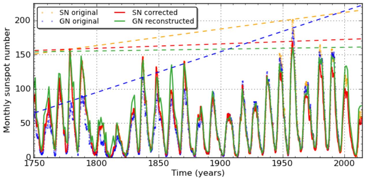
Sunspots are dark areas on the solar disc, characterized by strong magnetic fields that lower their temperature to about 4000 K compared to the surrounding 5800 K photosphere, making them appear as distinct darkening. [44] To repair this deficiency, Hoyt and Schatten introduced the Group Sunspot Number (\(G_N\)), which relies solely on the count of sunspot groups rather than individual spots, making the index compatible with earlier, less precise records and providing a more reliable reconstruction of solar activity back to the early seventeenth century. [62] However, methodological debates persist regarding the weighting schemes introduced by Wolf and modified by Waldmeier, which may have introduced systematic biases. Analysis of monthly values suggests that the group count and spot count are constrained to a narrow diagonal band, indicating that a one-dimensional relationship with the relative sunspot number might be sufficient for correction to an un-weighted value. [144][113][145] By calculating a logarithmic weight factor from the observed sunspot number, researchers can divide the International Sunspot Number since 2003 by this computed factor. [144] This supports the assertion that the weight factor function is also valid for the Waldmeier era at Zürich, allowing for the correction of the Zürich sunspot number for the inflation introduced by the weighting scheme. [117] It is important to take into account that the weight factor varies with the sunspot number itself, so one cannot use a constant weight factor throughout except as a first, crude approximation. [144] This update confirms that the previous series contained artificial trends that distorted the true amplitude of solar cycles, particularly in the modern era. [62] To resolve this, the solar community undertook a decade-long effort involving four Sunspot Number Workshops from 2011–2014, producing major recalibrations: \(S_{N}(1)\) became \(S_{N}(2)\) by Clette and Lefèvre, and HoSc98 became SvSc16 by Svalgaard and Schatten. [146] To address these issues, researchers have replaced the sunspot number between the years 1639 and 1715 with a reconstruction by Vaquero et al., which accounts for the large amount of missing sunspot number data and the difficulty in calibrating between different observatories. [147] While the International and Group sunspot numbers share similarities, such as indicating low activity during the Dalton minimum and a peak around 1957/58, they diverge sharply for earlier periods, with Group numbers running 25-50% lower than International numbers before 1882. [148] This divergence establishes that different sunspot series agree closely over the twentieth century but diverge significantly for earlier centuries. The consensus among diverse reconstructions since 1900, where underlying data are plentiful and of good quality, confirms that all methods are equally satisfactory provided the reference observer records are stable. [116][116][148][64] However, going back in time to Solar Cycle 11, peaking in 1870, the disagreement persists for all earlier cycles, highlighting the critical need for careful calibration when interpreting long-term solar variability from the limited observational records of the past.
The historical record of solar activity reveals a critical divergence in data quality as we look further back in time, particularly concerning the Maunder minimum period from 1645 to 1715. [62] Consequently, the Wolf series cannot reliably capture the true magnitude of solar cycles from 1650 to 1700, where the low fraction of active days indicates very low cycle amplitudes. In contrast, the Group Sunspot Number reconstruction, which relies on counting only the number of sunspot groups rather than individual spots, provides a more robust framework for this period. For instance, observations by Anton Maria Schyrlaeus Rheita in 1642 were initially misinterpreted as showing eight sunspot groups, but were later corrected to report one group in June, highlighting the pitfalls of early data interpretation. [30] Thus, the Maunder minimum is not merely a gap in the Wolf record but a period where the Group Sunspot Number provides the only reliable window into solar behavior, establishing a clearer picture of solar minima that extends back to the early 17th century.
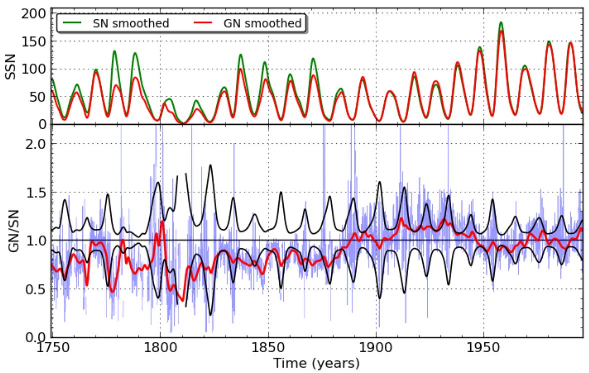
For the purposes of this book we adopt the SILSO Sunspot Number version 2.0 as the reference series. The 2015 recalibration corrected the long-standing Waldmeier discontinuity and remains the community standard maintained by the World Data Center in Brussels; where later analyses dispute particular segments of the record, we flag the disagreement rather than silently switching series. [146]
3.4 The Satellite Era TSI Record
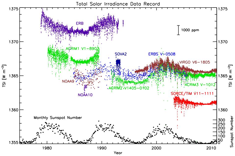
The satellite-era record of Total Solar Irradiance (TSI), the spatially and spectrally integrated radiant energy from the Sun at one astronomical unit, represents the primary energy input to the Earth’s climate system, dwarfing all other sources by a factor of three thousand. [149] These measurements rely on electrical-substitution radiometers, instruments that achieve high accuracy by modulating heater power to maintain thermal stability, thereby ensuring precise quantification of the incoming solar flux. Early instruments, such as ERB and ACRIM-1, initially measured higher TSI values than subsequent sensors like ERBE, ACRIM-2, and VIRGO, creating a divergence in the long-term record that has fueled ongoing debate regarding decadal trends. [149] The launch of the Total Irradiance Monitor (TIM) onboard the Solar Radiation and Climate Experiment (SORCE) mission introduced significant improvements in measurement accuracy and stability, ultimately establishing a lower, now internationally accepted TSI value of approximately 1361 W m⁻². [149] Despite these advancements, the composite TSI record remains subject to scrutiny, particularly concerning the gap-bridging methods used to reconcile data from different instruments. [150] This uncertainty is critical for climate studies, as it directly impacts assessments of solar forcing on global temperatures. [150] The launch of the SOlar Radiation and Climate Experiment/Total Irradiance Monitor (SORCE/TIM) helped resolve this offset issue. [149] It confirmed lower TSI values and indicated that predecessor instruments were approximately 0.35% erroneously high. [149] Subsequent corrections were retroactively applied to flight data for ACRIM3 and VIRGO. [149] The lower TSI value established by SORCE/TIM was validated by later missions, including the Total Spectral and Solar Irradiance Sensor (TSIS-1)/TIM, and is now the accepted value by the International Astronomical Union. [149] This recalibration improved uncertainties regarding Earth’s energy balance by resolving discrepancies between incoming and outgoing radiation. [149]
The satellite-era record of total solar irradiance (TSI) reveals significant discrepancies in long-term trends depending on the composite method employed. [86] The ACRIM composite suggests TSI increased during the 1980s and 1990s but has slightly declined since then. This upward pattern from 1980 to 2000 stands in stark contrast to the PMOD composite, which indicates a slight downward trend over the same period. [100][101][100] The multi-decadal trending difference between these composites is crucial for discriminating among solar models used to interpret climate changes. [86] If TSI increased from 1980 to 2000, total solar and heliospheric activity could have increased as well, potentially contributing significantly to the global warming observed from 1980 to 2000. [86] Consequently, the choice of composite directly impacts assessments of solar forcing, with the ACRIM data supporting the possibility that TSI acted as a primary driver of global temperatures during this interval, whereas the PMOD data suggests a different mechanism for the observed warming.
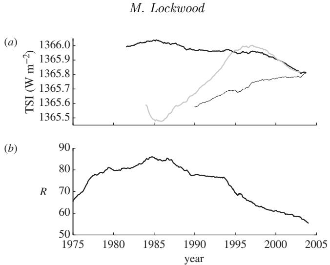
The satellite-era record of Total Solar Irradiance (TSI) reveals significant discrepancies in how long-term trends are reconstructed, particularly concerning the period known as the ACRIM Gap — the roughly two-year hiatus (1989–1991) between the ACRIM1 and ACRIM2 satellite radiometers, which every composite must bridge with lower-precision instruments. [86] During the 1990–1992.5 interval, comparisons between the WSKF06 proxy models and the PMOD composite highlight a fundamental divergence in data processing. [86] While the WSKF06 models show stationarity, the PMOD composite exhibits a significant downward trending difference, largely due to Fröhlich’s downward adjustment of the ERB data. [86] This adjustment involved a shift of approximately 0.86 W/m², which is more than twice the shift derived from WSKF06 comparisons. [86] Consequently, the resulting PMOD composite suggests that TSI has been steadily decreasing since at least the late-1970s, a conclusion that stands in contrast to the ACRIM composite, which would require an upward adjustment of ~0.46 W/m² to reconcile the minima trends. This ongoing debate over gap-bridging methods underscores the uncertainty in decadal TSI trends, as the choice of composite directly influences the perceived direction of solar output over recent decades. This methodological sensitivity implies that the magnitude of solar forcing in climate models remains somewhat ambiguous. [51][101][100][100] Consequently, attributing specific temperature variations to TSI fluctuations requires careful consideration of these reconstruction uncertainties.
The divergence between the ACRIM and PMOD total solar irradiance composites stems from how the ACRIM Gap is bridged using conflicting ERB and ERBE trends. This discrepancy suggests that the resulting long-term solar trends may be somewhat ambiguous. [86]
Since 1978, direct observations of Total Solar Irradiance (TSI) have been obtained from Earth-orbiting satellites, providing a continuous time series of the integrated radiant energy arriving at the top of Earth’s atmosphere. [150] However, because these instruments wear out and must be replaced, the records from each mission require inter-calibration to bridge data gaps and account for instrument degradation. Consequently, the magnitude of secular TSI change over the satellite period remains uncertain due to inconsistencies in cross-calibration. While satellite data demonstrate that TSI varies by as much as 0.05–0.07% over an 11-year solar cycle, determining any multi-decadal trend beyond this cycle is difficult. [64][151][64][149][100][101] These variations illustrate the difficulties faced when combining experiments, suggesting that it is currently not possible to be confident of any multi-decadal trend in TSI. [150]
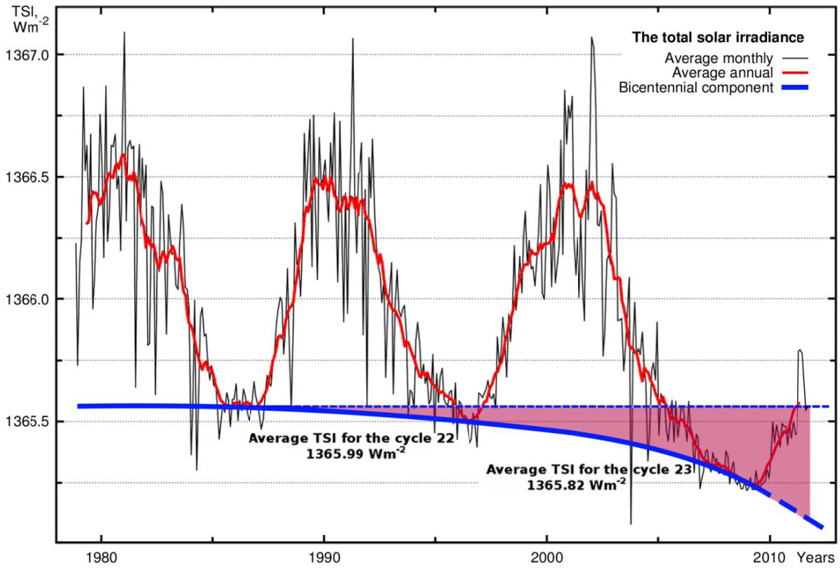
The satellite era, which began in late 1978, provides the only direct observations of Total Solar Irradiance (TSI), the integrated radiant energy arriving from the Sun at the top of Earth’s atmosphere. [86] However, due to data gaps and instrument degradation, the precise calibration needed to bridge these records is not universally agreed upon, leading to divergent composites. For instance, early instruments like ERB and ACRIM-1 measured higher TSI values than subsequent instruments, a discrepancy that was partially resolved following the SORCE/TIM launch and international calibration workshops, which established a lower accepted TSI value of approximately 1361 W m⁻². [149] Satellite data demonstrate that TSI varies by as much as 0.05–0.07% over an 11-year solar cycle, amounting to around 1 W/m² at the top of the atmosphere and only 0.2 W/m² at the surface after accounting for geometry and albedo. [150] The critical question for climate science is whether there is a trend in the TSI data beyond this 11-year cycle, as this could have implications for estimates of TSI changes on long timescales. [150] Consequently, the debate over whether TSI has increased or decreased over the multi-decadal scale remains unresolved, with reconstructions from different groups disagreeing on the magnitude and direction of any potential trend.
3.5 F10.7 and the Modern Activity Index
The F10.7 index — a daily measure of the Sun’s radio emission at the 10.7 cm wavelength, which rises and falls with the amount of magnetically heated plasma in the upper solar atmosphere — has been recorded continuously since February 1947, creating a consistent dataset that allows researchers to track solar cycles with high precision. [44]
The Sun’s radio flux density at the 10.7 cm wavelength serves as a critical metric for solar activity, distinct from visible sunspot counts. [130]
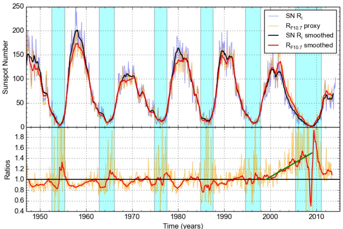
The 10.7 cm Solar Flux, measured daily by the Canadian Solar Radio Monitoring Programme since 1946, offers a completely objective record of solar activity that can be taken under virtually all weather conditions. [130] While this radio flux is highly correlated with the International Sunspot Number, the relationship between the two indices is slightly nonlinear, with the slope changing as the sunspot number increases up to about 30. This complexity is captured by the Holland and Vaughn formula, which accounts for the base level of about 67 solar flux units and the varying sensitivity at different activity levels. [146][130][130][154][148] Although the two measures are tightly linked, the 10.7 cm radio flux lags behind the sunspot number by about one month, adding a temporal nuance to the correlation. [130]
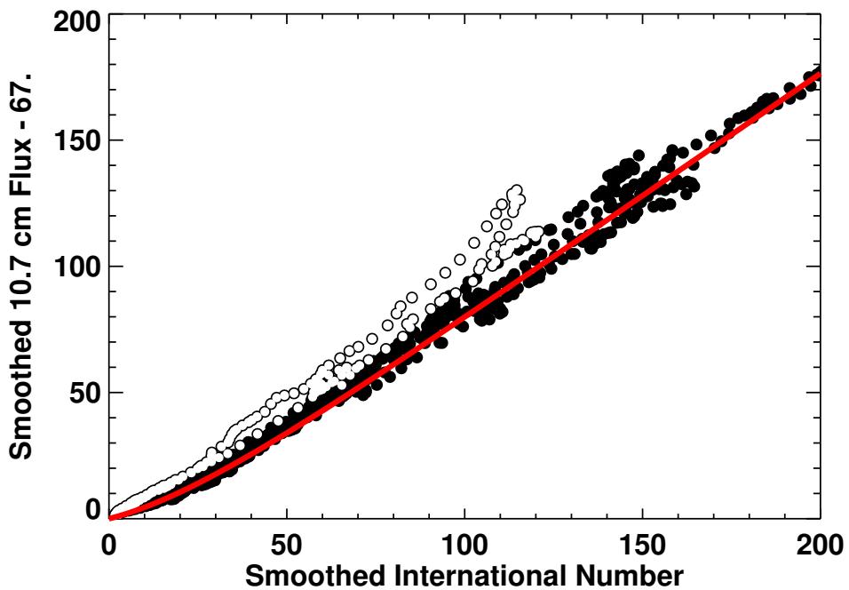
The 10.7 cm Solar Flux, measured daily by the Canadian Solar Radio Monitoring Programme since 1946, offers a completely objective measure of solar activity that can be recorded under virtually all weather conditions. [130] Unlike sunspot counts, which rely on visual observation, this radio flux captures disc-integrated emission at 2800 MHz, providing a stable baseline of about 67 solar flux units for a quiet Sun. [130] The relationship between this radio index and the International Sunspot Number is remarkably tight; statistical analysis confirms that the two measures are highly correlated, with a correlation coefficient of r = 0.995. This near-perfect linear alignment demonstrates that F10.7 serves as a robust proxy for overall solar variability, tracking the rise and fall of solar cycles with precision. [155][146][130][156][157][158]