7 The Underground Connection: Volcanism and the Sun
Grand minima have coincided with anomalously intense volcanism; plausible mechanisms — lithospheric stress, isostatic rebound, deep-Earth degassing — are testable and matter for the coming minimum.
7.1 When the Sun Goes Quiet the Earth Gets Loud
By analyzing carbon-14 derived from tree rings and beryllium-10 extracted from Greenland and Antarctic ice cores, researchers have established that solar activity exhibits long-term variability, including periods of significantly reduced activity known as grand minima. These isotopic archives serve as proxies for cosmic-ray flux, which increases when the Sun’s magnetic shielding weakens during quiet phases. [56][46][46][250][65] This increased cosmic-ray flux is not merely a theoretical construct but a measurable phenomenon captured in geological archives, providing a baseline for understanding solar-climate interactions. [251] The consistency of these signals across different isotopes and geographic locations suggests that regional anomalies are not the primary driver, indicating that the observed variations are global in scale and linked to solar modulation. [244] The Maunder Minimum, for instance, is characterized by a distinct lack of visible sunspots and a corresponding spike in radionuclide production, offering a signature of reduced solar activity. [44]
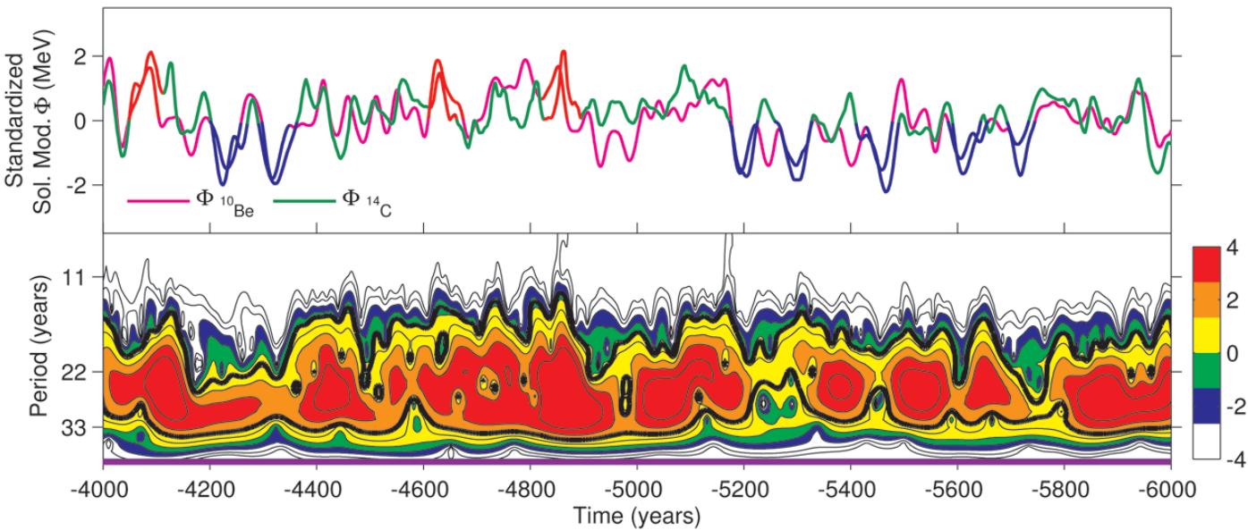
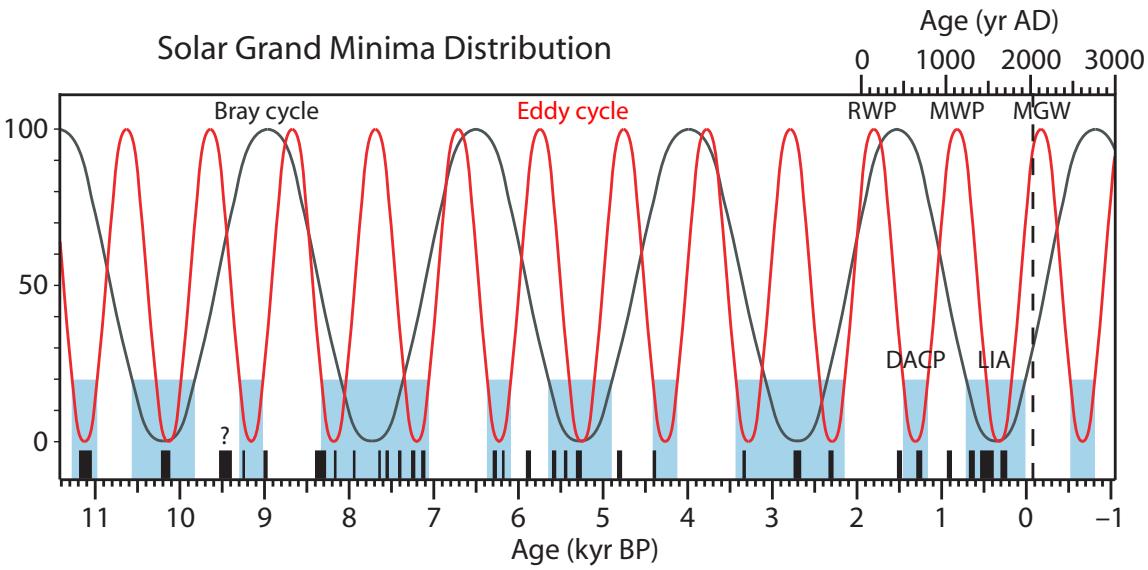
Holocene reconstructions indicate that grand minima are not periodic but appear as the result of chaotic or stochastic processes within clusters separated by 2000–2500 years. Analysis of radiocarbon data reveals a weak, marginally significant quasi-periodicity of 2000–2400 years, a well-known period in \({}^{14}\)C records that likely relates to the clustering of grand minima rather than to a long-term modulation of solar activity. [33][1][156][211] This pattern suggests that the occurrence of grand minima and maxima is defined by stochastic or chaotic processes, with no clear periodicities observed in the occurrence of grand maxima. [252] The observed effect of the 2500-year Bray solar cycle is to result in long Spörer-type solar grand minima or clusters of such minima at its lows. [211] These climatic shifts, registered mainly as significant reductions in winter temperatures and increases in precipitation in the North Atlantic region, have historically coincided with societal disruptions, including food crises and population decreases. [211] The biological and temperature subdivisions of the Holocene display transitions related to the lows of the Bray cycle, suggesting that climate-related disruptions have been quasi-periodic drivers of societal change. [211] Thus, while the timing of individual grand minima may be stochastic, their clustering within the broader 2000–2500 year cycle provides a structural framework for understanding long-term solar variability and its associated climatic impacts.
Reconstructions of solar activity during the Holocene period, spanning from 10,000 B.C. to the present, reveal that the Sun exhibits great variability in the strength of each solar cycle. [1] While some cycles produce a high number of sunspots, others result in low numbers, leading to distinct epochs of suppressed activity known as solar Grand Minima. [253] A solar Grand Minima is defined as a period when the (smoothed) sunspot number is less than 15 during at least two consecutive decades. [252] Detailed analysis of these reconstructions shows that the Sun spends about 17 percent of the time in a Grand Minima state. This finding suggests that grand minima are not rare anomalies but a recurring feature of solar behavior over the past ten millennia. [111][1] In contrast, energetic solar Grand Maxima states are typically short-lived, lasting in the order of 50 years.
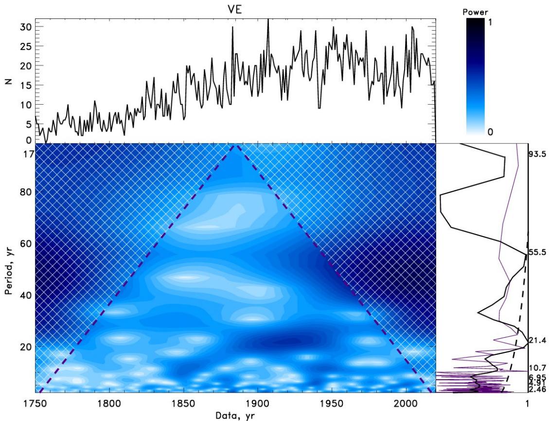
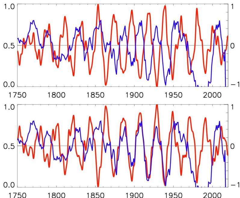
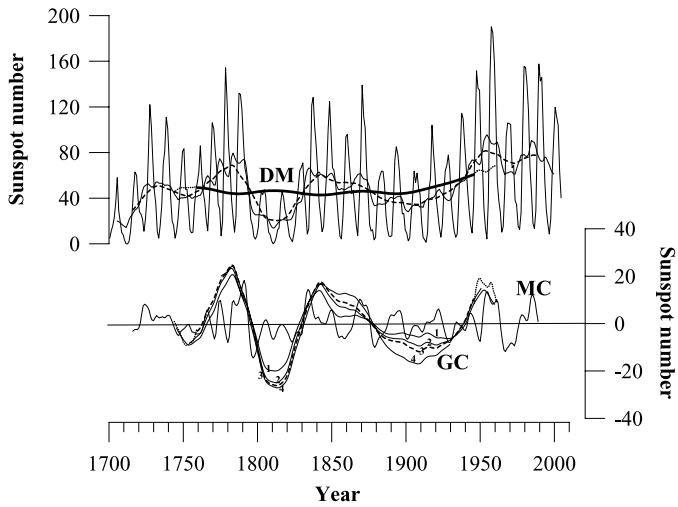
The sunspot number records establish a solar quasi-period of 90 ± 10 years, known as the Wolf-Gleissberg cycle, as the most prominent of the longer solar cycles. This periodicity is supported by wavelet power spectrum analysis of sunspot data from 1700 to 2020, which yields a mean total wavelet period of Tsa = 4*22.5 = 90.0 years. [253][215][19][254] Fast Fourier Transform (FFT) computations on the full sunspot number time series, including subsets of the first half, second half, and middle half, reveal that the 87.6-year Gleissberg peak is sharp and prevalent across all intervals, although it is absent in recent data. [123] While earlier hypotheses, such as those by Stothers, suggested an 11-year periodicity in volcanic activity, recent analyses of 3,829 eruptions with a Volcanic Explosivity Index (VEI) of 2 or greater reveal a dominant 22-year period that aligns with the solar background magnetic field (SBMF) cycle. [254] Specifically, the evidence suggests that more volcanic eruptions occur during the maximum phases of the doubled solar cycles when the solar background magnetic field possesses a southern polarity. [181] This correlation is not uniform across all historical periods; a rather high positive correlation between the number of volcanic eruptions and the southern polarity of the SBMF was established for the period 1868–1950, whereas a much smaller negative correlation was observed during 1750–1868. [11] The proposed link involves increased electromagnetic interaction between the SBMF and the terrestrial magnetic field, causing geomagnetic disturbances that can lead to shifts of the crusts, most powerful earthquakes, and volcanic eruptions. [255] The reduced correlation between volcanic eruptions and solar activity indices recorded during the period 1750–1868 can be associated with a geomagnetic jerk and the related migration of the North pole towards lower latitudes. [255] Differences in eruption frequencies over the phases of solar cycles may also relate to differences in solar activity indices defined by sunspots and eigen vectors of magnetic fields related to different types of solar magnetic fields, specifically the toroidal and poloidal fields. [181] The lack of correlation in the period 1950–1980 is linked to open air nuclear bomb testings that distorted the effects of the solar magnetic field. [181] In summary, the increase of volcanic eruptions established during solar cycles with the southern polarity of the SBMF emphasizes the importance of solar-terrestrial interaction in volcanic eruptions. [254] Hence, despite links between volcano occurrences and solar activity not being clear yet, the consequences of volcanic eruptions for the terrestrial atmosphere during cycle 26 with the southern polarity of the solar magnetic field can be expected to be noticeable during the modern Grand Solar Minimum (2020–2053).
7.2 The Maunder Era Eruptions
This event, which began on February 19 and continued until mid-March, stands out as the largest historical explosive event in the Andes, classified as VEI 6. The eruption’s magnitude is confirmed by the correlation of geologic evidence with early Spanish chronicles, which document a sustained Plinian column reaching 27–35 km in height and delivering a dacitic pumice fall with a dense rock equivalent volume of 3.1 km³. [256][257][258][259] Ash fall was reported 200–500 km away in south Peru, west Bolivia, and north Chile, while strong winds carried fine ash more than 500 km to the west and into the Pacific Ocean. [256] The onset of this high-discharge eruption was fueled by the disruption of an active hydrothermal system enclosed in the pre-AD 1600 amphitheater, with computed volumetric eruption rates between 5.4–6.6 × 10⁴ and 1 × 10⁵ m³/s. [256] The preservation of tephra-fall deposits in the arid and semi-arid environments of the Central Andes provides a critical archive for understanding the dispersal and impact of these massive explosive events. [257] From 260 thickness measurements of the plinian pumice fall made over an area of approximately 95,000 km², they surmised a reconstructed 7.87-km³ bulk volume of the plinian pumice-fall deposit. [256] This figure was considered potentially underestimated beyond the 1-cm-isopach. [256] Adding the volume of post-plinian tephra to that of the plinian pumice fall led to a total bulk volume of 11.4–12.1 km³. [256] The chemical composition of glass in juvenile tephra was also examined, linking it to glass in the Antarctic ice. [260]
The chemical characteristics of juvenile tephra from the AD 1600 Huaynaputina eruption allow a firm cause–effect link to be established with glass found in Antarctic ice, improving estimates of stratospheric loading. [260]
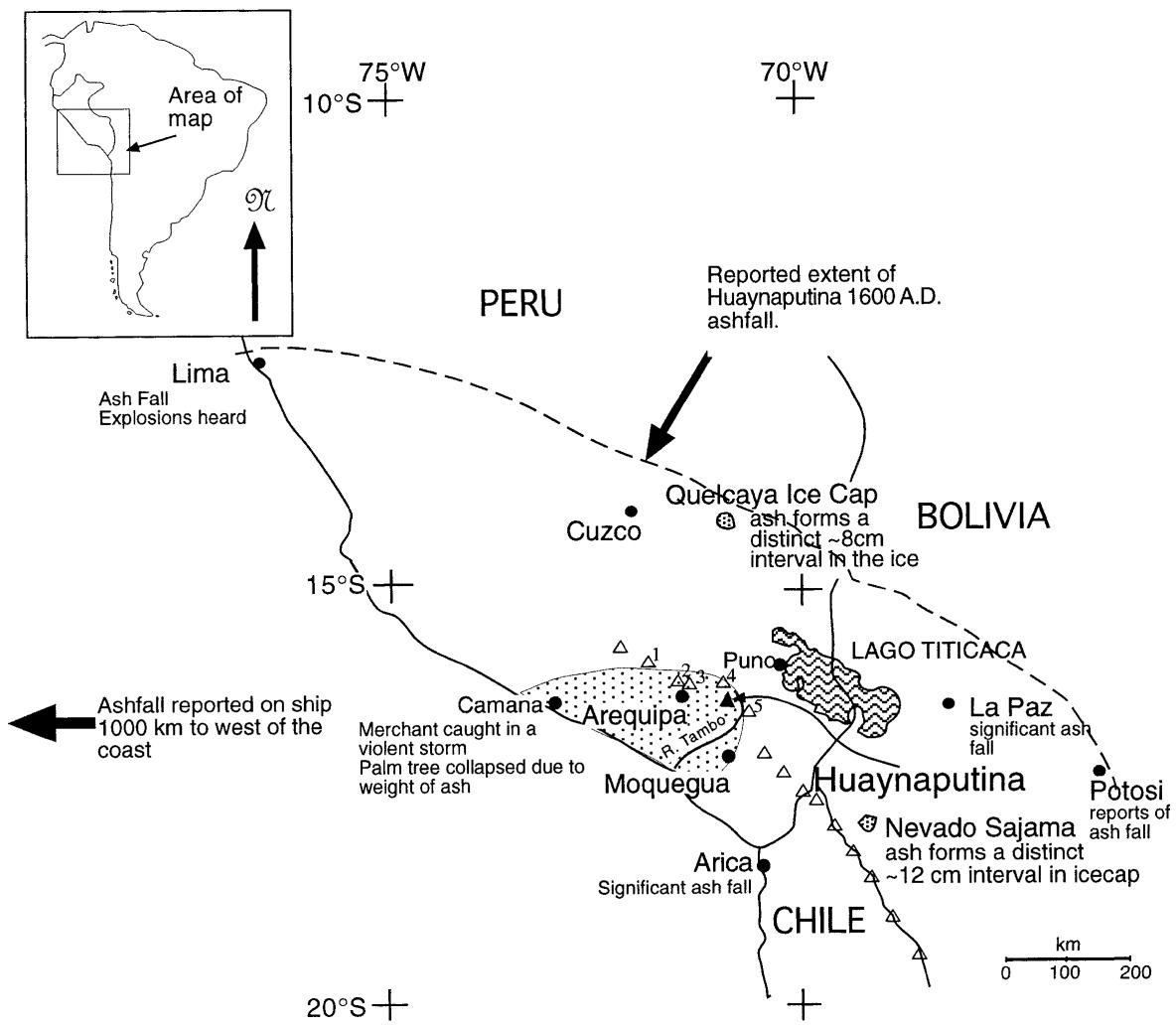
The AD1600 eruption of Huaynaputina in southern Peru stands as one of the largest explosive events in historic times, with tephra deposits and juvenile glass chemistry establishing a firm cause–effect link to acidity spikes in Antarctic ice. [260] This stratospheric loading suggests statistically significant global cooling, consistent with the severe climatic anomalies recorded across multiple proxy datasets in the immediate aftermath. [260] Tree-ring chronologies from the Swiss and Austrian Alps, along with maximum latewood density data from thirteen sites along the northern tree line of North America, indicate extremely low temperatures in 1601 AD. [261] Significant frost and light rings identified in western USA, near Bush Lake in Canada, and in the Polar Urals further support this widespread cooling signal. [262] Historical records corroborate these biological proxies, noting an unusually cold summer in England and Italy, a severe winter in Russia, Latvia, and Estonia, and widespread crop failures in northern China due to killing frost. [261]
The ecological aftermath of the AD 1600 Huaynaputina eruption provides a precise chronometer for studying rapid biological colonization in the northern Atacama desert. [263] On the deep pumice substrates near Omate, Moquegua, Peru, floristic inventories demonstrate that approximately 59 angiosperm species established themselves within the last 400 years. This unique vegetation type, dominated by therophytes and chamaephytes, exhibits a floristic composition with the highest similarity to the coastal Lomas de Tacna rather than geographically closer Sierra formations, despite stark climatic differences. [263][264] The presence of nine species representing highly disjunct populations, with nearest living relatives located 200 to over 700 km away, confirms that long-distance dispersal events were the primary colonization mechanism on the denuded substrate. [263] Morphological analysis further establishes that four taxa have undergone considerable divergence from their source populations, with two potentially representing neoendemics, proving that speciation can occur rapidly on suitable target areas. [263] These findings highlight how the specific edaphic and climatic filters of the Omate pumice slopes precluded establishment from adjoining habitats while allowing successful colonization from remote source areas, offering insights into the speed of phyto-diversity processes following major explosive volcanic events. [263]
The ecological aftermath of the 1600 AD Huaynaputina eruption provides a unique natural laboratory for studying rapid colonization on deep pumice substrates in the northern Atacama desert. [263] Research into the vascular plants establishing themselves on the Huaynaputina pumice slopes near Omate, Moquegua, Peru, reveals a distinct floristic composition that has developed over the last 400 years. [263] Floristic composition on Huaynaputina slopes shows highest similarity to the coastal Lomas de Tacna rather than geographically closer Sierra formations. This finding is quantified by a Sørensen index of 24 at the species level between the Omate sites and the Lomas de Tacna, a similarity nearly twice that of any other compared sites. [263][263] The porous pumice absorbs precipitation only in upper layers, keeping subsoil dry year-round, which mimics the climatic constraints of the coastal Lomas rather than the moisture-retaining Sierra soils. [263] Consequently, the Lomas vegetation serves as the natural recruiting ground for this unique Andean vegetation type, despite the significant altitudinal and geographical barriers. This strong ecological link demonstrates how specific substrate properties can override proximity in determining post-eruption flora, highlighting the role of long-distance dispersal mechanisms in repopulating denuded volcanic landscapes. [264] Crucially, nine species on these slopes represent highly disjunct populations, with their nearest known living populations located 200 to greater than 700 kilometers away in central Peru, Chile, Bolivia, or Argentina. These disjunctions suggest recent long-distance dispersal as the primary colonization mechanism, given that the substrate was denuded in 1600 AD. [263] Abiotic conditions, including soil type and climate, appear to limit establishment from neighboring vegetation. [263] Morphological analysis reveals that four taxa exhibit clear differences from populations elsewhere, with two potentially representing neoendemics, indicating rapid morphological divergence over the 400-year period. [263] Rodent midden data suggest no dramatic late Holocene climatic changes since 1600 AD, though a strong El Niño event in 1652 AD may have facilitated Lomas flora expansion and subsequent dispersal to Omate. [263] This young, annual-dominated community contrasts with the shrub-dominated flora on adjacent rocky soils, identifying the Omate pumice slopes as the first recorded Andean vegetation type dominated by annuals and floristically akin to coastal Lomas. This unique assemblage likely reflects a specific post-eruption colonization trajectory rather than a stable equilibrium state. [263] Consequently, the site serves as a critical natural experiment for understanding rapid ecological succession in extreme volcanic environments.
7.3 Tambora and the Year Without a Summer
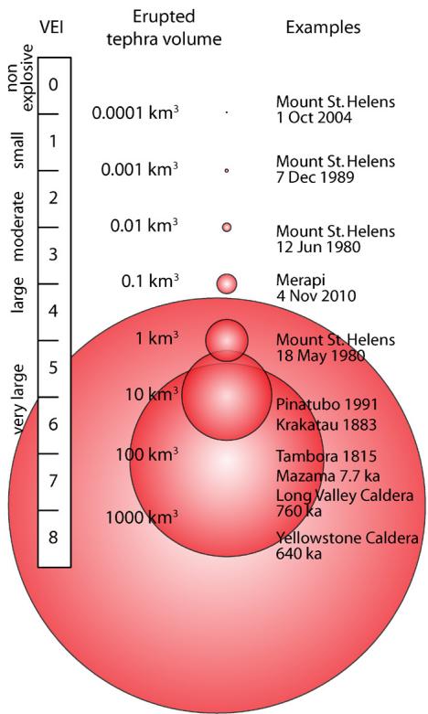
The April 1815 eruption of Mount Tambora stands as a defining event in the instrumental record, classified at an intensity of 7 on the volcanic explosivity index, a relative measure of volcanic explosiveness that ranges from 0 to 8. [265] This aerosol umbrella, six times the size of Mount Pinatubo’s 1991 cloud, disrupted normal patterns of temperature and precipitation across the hemispheres by entering the meridional currents of the global climate system. [83] The subsequent year of 1816 has been termed the “Year Without a Summer,” a period marked by significant climate anomalies and harvest failures across Europe and North America. [266] The dust veil increased visual extinction in the stratosphere by 1.4 ± 0.2 mag at northern middle latitudes, implying a worldwide stratospheric aerosol load of ~2.0 × 10^14 g, in near agreement with values estimated from Greenland ice acidities. [80] The relation between volcanism and climate depends on eruptive scale, with volcanic ejecta and gases penetrating high enough to reach the stratosphere where sulfate aerosols form and spread aloft by winds and meridional currents. [83] The telltale sulfate imprint left on the ice for paleoclimatologists to discover more than a century and a half later confirms the global reach of this atmospheric perturbation. [267]
The 1815 eruption of Mt. Tambora discharged approximately 150 km³ of ash and pumice — about 50 km³ of dense-rock-equivalent magma, creating a dust veil that increased visual extinction by 1.4 ± 0.2 magnitudes at northern middle latitudes. [80] These stratospheric sulfate aerosols scattered incoming solar radiation, establishing a global cooling of approximately 0.4 to 0.8°C during 1815–1818. The climatic anomalies were particularly severe in eastern North America and central and western Europe, where persistently cold and wet weather defined the late spring and summer of 1816. [268][80][75] This period, known as the “Year Without A Summer,” caused significant socio-economic impacts, including severe famine, and was perceived by contemporary populations as a catastrophic event. [269] While the Dalton Minimum contributed a small additional cooling effect, the primary driver was the volcanic forcing. [85] The magnitude of Tambora’s impact, exceeding any other known eruption in the past 10,000 years, provides a high-accuracy calibration standard for investigating earlier explosive volcanic events. [80] These conditions caused widespread crop failures, leading to famine and social distress compounded by the aftermath of the Napoleonic wars. [269] This cooling is further evidenced by climatic indicators such as late grape harvests in France and frost damage rings in trees in the western United States and South Africa. [75] The dot marks Geneva, located within a region of negative SLP anomaly. [270]
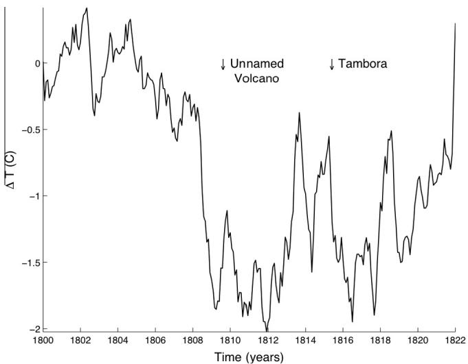
The summer of 1816 in western Europe was cool and exceedingly wet, a condition that compounded the aftereffects of the Napoleonic Wars to produce famine, disease, and social unrest. [75] Data from Manley show that the summer months of 1816 in central England were about 1.5°C cooler than during the summer of 1815, while pressure anomaly charts reconstructed by Kelly et al are dominated by negative pressure anomalies over Europe beginning in early 1816. [75] This atmospheric shift led to a southward track for middle-latitude cyclones, creating a cold, wet summer centered over England and extending across much of western Europe. [83] In North America, records from Hudson’s Bay Company posts on the eastern side of Hudson Bay indicate that the summers of 1816 and 1817 were the coldest in the modern record, a finding supported by tree-ring data from northern and western Quebec. [75] The summer of 1816 was the coldest in New Haven, Connecticut, for the entire period from 1780 to 1968. [266] Repeated frosts in New England during late spring through summer caused severe crop failures, resulting in poor harvests and food shortages. [82] Indian corn in Pennsylvania rotted on the stock, frozen hard by the cold, while newspapers from England noted that 1816 was a year in which there was no summer. [40] These widespread crop failures, particularly of corn in America and grain in Europe, demonstrate the devastating impact of the 1816 climate anomalies. Consequently, the resulting socioeconomic disruptions appear to have been significantly exacerbated by these climatic conditions. [271][75][40][83]
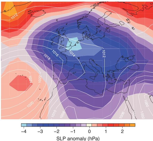
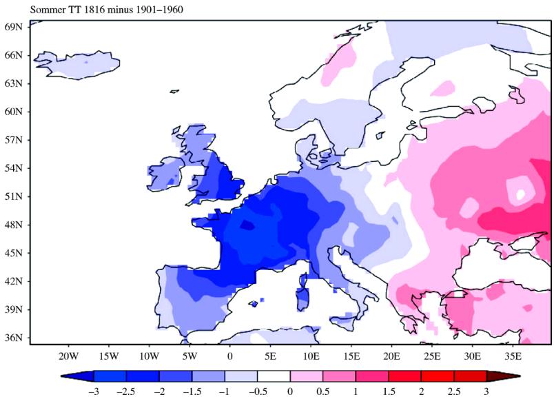
The summer of 1816 in western Europe was cool and exceedingly wet, a condition that compounded the aftereffects of the Napoleonic Wars to produce famine, disease, and social unrest. [75] This period, referred to by Post as “The Last Great Subsistence Crisis in the Western World,” saw negative pressure anomalies dominate Europe beginning in early 1816, leading to a southward shift in middle-latitude cyclone tracks. [75] Data from Manley indicate that the summer months of 1816 in central England were about 1.5°C cooler than during the summer of 1815. [75] In North America, records from Hudson’s Bay Company posts on the eastern side of Hudson Bay show that the summers of 1816 and 1817 were the coldest of any in the modern record, a finding supported by tree-ring data from northern and western Quebec. [75] Repeated frosts in New England caused crop failures, resulting in poor harvests and food shortages. [82] The resulting food insecurity and social distress following the 1816 harvest failures contributed to outbreaks of typhus and other diseases in Europe. [269] At the height of the typhus epidemic in September 1817, Dublin doctors warned of impending ruin, while the medical establishment in Edinburgh expressed alarm at the continued fever spreading across the British Isles. [83] This anomalous cooling followed the spectacular April 1815 eruption of Tambora volcano on Sumbawa Island in Indonesia, which ejected approximately 150 km³ of ash and pumice, equivalent to about 50 km³ of dense rock equivalent magma, into the atmosphere. [75] The eruption column reached an estimated 50 km into the stratosphere, dispersing ash over an area exceeding 4 × 10⁵ km² and causing darkness for up to two days at distances of 600 km from the source. [75] However, the severity of the 1816 cooling cannot be attributed to Tambora alone. Crucially, European temperature measurements during the Dalton Minimum showed a decline in place well before the Tambora eruption, with the lowest temperatures recorded prior to 1816 according to the European temperature profile done by David Archibald in his work, The Past and Future Climate.
7.4 Hunga Tonga the Eruption That Warmed the World
The January 2022 eruption of the Hunga Tonga–Hunga Ha’apai volcano represents a singular event in the modern observational record, distinguished not by sulfur dioxide but by an unprecedented injection of water vapour into the stratosphere. Satellite observations from the NASA Aura satellite and balloon data collected by the National Oceanic and Atmospheric Administration (NOAA) near Reunion Island confirm that approximately 150 Tg of water vapour was blasted roughly 60 km into the air, increasing the existing global stratospheric burden by 10% — the largest stratospheric perturbation of water vapour observed in the satellite era, which spans more than 30 years.[274][275][276] While classic explosive eruptions like Pinatubo or Tambora are defined by their sulfate aerosol loads, which scatter sunlight and induce a temporary cooling effect, Hunga’s primary radiative forcing agent was water. The immediate atmospheric response included strong cooling in the Southern Hemisphere mid-latitude stratosphere, which strengthened the mid-latitude jet and slowed the Brewer–Dobson Circulation, while simultaneously perturbing polar ozone chemistry through increased HOx and polar stratospheric cloud formation. Satellite records show the dark patch of high humidity spreading globally from the Southern Hemisphere to the north over the course of a year.
What made Hunga different was the ratio of water to sulfur. TROPOMI satellite-based measurements of SO₂ concentrations in the atmosphere establish that the total stratospheric SO₂ mass was approximately 0.4 Tg, a figure consistent with other estimates of ~0.5 Tg that confirm the eruption injected only a modest amount of sulfur dioxide.[277][276][278] This disparity is critical because SO₂ oxidizes into sulfate aerosols that reflect sunlight and cool the surface, whereas stratospheric water vapour acts as a greenhouse gas that warms it. Atmospheric physics demonstrates that stratospheric water vapour effectively alters radiative forcing and influences global surface temperature once it enters the stratosphere.[1][279][276][280][181] Consequently, the Hunga event produced a transient natural warming pulse rather than the classic volcanic winter associated with Pinatubo-type eruptions — a thermal anomaly that acted in direct opposition to the traditional volcanic winter narrative.
How long will the pulse last? In the first two years post-eruption, the stratospheric burden hardly changed, leaving the residence time of the volcanically injected water vapour uncertain, and early estimates varied widely — some projections suggested a return to baseline conditions as early as 2025, while others predicted a lingering presence for more than a decade. The Microwave Limb Sounder (MLS) instrument aboard NASA’s Aura satellite, however, has provided continuous, high-resolution observations of the Hunga-enhanced water since the eruption, and recent data show a substantial decline from 2024 to early 2025, marking the largest drop since the event. Comparison with 3-D numerical model simulations demonstrates that the long-term removal of the Hunga water has entered a new phase, with stratosphere-troposphere exchange playing an increasingly important role, exceeding Antarctic dehydration in 2024. The primary sinks for this excess water include ice polar stratospheric cloud sedimentation and stratosphere-to-troposphere transport in middle-to-high latitudes, with additional minor loss in the mesosphere due to photolysis. The additional stratospheric water vapour is now decaying steadily with an e-folding time of 3 years, a trajectory that will bring the perturbation back within the observed pre-Hunga range of variability around 2030 — quantifying the residence time of the Hunga stratospheric water vapour perturbation at 9 years.[276] The decay estimate is statistically well-constrained: combining the formal fitting uncertainty of the exponential fit to the MLS time series through July 2025 with the spread arising from natural variability yields a total two-sigma uncertainty of roughly 0.29 years.
This transient natural warming pulse contributed to the global temperature surge observed in 2023 and 2024, challenging narratives that attribute recent heat solely to anthropogenic carbon dioxide. Unlike the persistent cooling shadow cast by sulfate aerosols, which can linger for years and mask underlying solar trends, the radiative impact of stratospheric water vapour is inherently temporary, governed by the atmospheric residence time of the molecule itself. As the vapour dissipates toward 2030, the radiative forcing will wane, allowing the underlying climate drivers — solar irradiance and cosmic-ray modulation among them — to reassert their influence on global surface temperatures. Understanding the timeline of this decay is critical for disentangling natural variability from long-term climate trends, particularly in assessing the compounding effects of solar minima and volcanic activity.
7.5 Mechanisms Why Might the Sun Affect the Earth S Crust
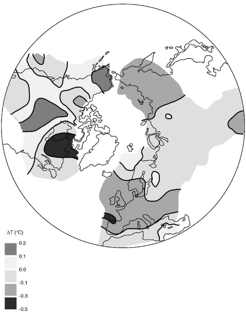
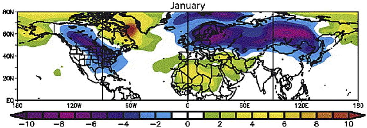
In the 1970s, John Eddy noticed a correlation between solar activity and the European climate over the previous millennium, observing that the Little Ice Age (1300–1850 AD) was a cold period that took place while the Sun was particularly inactive, whereas the Medieval Warm Period (1000–1200 AD) occurred while the Sun was active. [64] A new reconstruction of temperature variability in the extratropical Northern Hemisphere during the last two millennia correlates reasonably well with the assumed low-frequency variability in solar forcing of the last millennium, revealing that several periods with especially low solar activity are visible in the reconstruction, including the Wolf Minimum (c. [2] AD 1645–1715). Figure 5a shows recent reconstructions of temperature variation over the last 1000 years, while Figure 5b displays cosmic ray reconstructions based on ice cores from Antarctica and an ice core from Greenland, demonstrating a remarkable correlation between the changes in temperature and changes in cosmic rays caused by solar activity. [64] Historical data associate the European Maunder Minimum winter cooling with enhanced northeasterly advection of continental air, consistent with an anomalous negative NAO, and reconstructions of large-scale surface temperature patterns from networks of diverse proxy information, such as tree rings, ice cores, corals, and historical records, provide empirical estimates of the large-scale climate response to solar forcing. [281] When filtered to isolate the multidecadal-to-centennial time scales associated with the Maunder Minimum, the empirical regression shows a clear AO/NAO-type pattern of alternating cold land and warm ocean temperature anomalies, indicating that solar forcing affects regional scales much more strongly than global or hemispheric scales. [281] Ocean sediments show a decreased SST of 1° to 2°C in the Sargasso Sea during the 16th to 19th centuries, which is consistent with a reduced NAO but not with uniform basin-wide cooling, while other evidence suggests colder North Atlantic temperatures during those centuries, including evidence for increased sea ice around Iceland. [281]
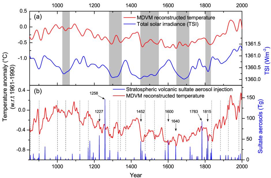
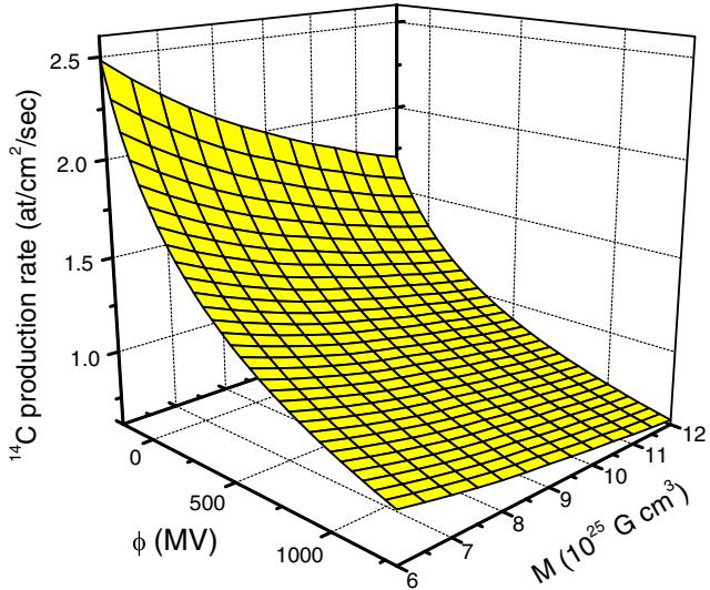
The proposed link between solar activity and climate hinges on a microphysical mechanism connecting cosmic ray ionization in the Earth’s atmosphere to cloud formation. [282] This relationship may provide an explanation for reported tropospheric and stratospheric oscillations, supporting the hypothesis that solar modulation of cosmic rays affects cloud cover and, consequently, the climate. [103] A comparison of this low-noise radionuclide production record with changes in the geomagnetic dipole field strength demonstrates that geomagnetic shielding is the primary driver of multimillennial variability, establishing that stronger geomagnetic fields correspond to lower cosmic radiation levels. While solar modulation dominates cosmic radiation variations on multidecadal to centennial time scales, as indicated by the coincidence of radiation maxima and grand solar minima, the influence of solar activity diminishes over longer periods. [56][225][11][215][283][181] Research at the GeoForschungsZentrum (GFZ) Potsdam provided fine detail of relative paleointensity variations, recording the magnetic field strength at the Kolbeinsey Ridge in the Iceland Sea over the past 300,000 years. [218] This data indicates that when the magnetic field is strong, it shields the Earth from galactic cosmic rays, whereas weak fields near reversals allow bombardment of equatorial regions. [218] Magnetostratigraphic studies established that the pattern of ice sheets in North America changed with each major reversal of the Earth’s magnetic field polarity, correlating with topographic changes. [284] Consequently, periods of geomagnetic field reversal roughly correspond to cold episodes in paleoclimatic reconstructions, though this correlation is not strong. A detailed study revealed a weak but persistent correlation between Northern hemisphere temperature and geomagnetic field intensity during the last millennium, implying that cosmic rays play a role in climate variations. [225] The last two interglacial periods ended abruptly when the magnetic field was weak and at the point of a reversal, approximately 70,000 and 180,000 years ago, suggesting that geomagnetic weakening can amplify global cooling effects. [218] The existence of a physical mechanism, which is sufficiently strong, indicates that the deduced inverse correlation between solar cycle length and long-term variations in global temperature may be related to long-term variations in the solar modulation of cosmic-ray flux. [103] Thus, the atmospheric evidence, though indirect, supports the broader thesis that solar variability plays a significant role in modulating Earth’s climate and geological activity.
7.6 What If the Next Minimum Brings the Next Big Eruption
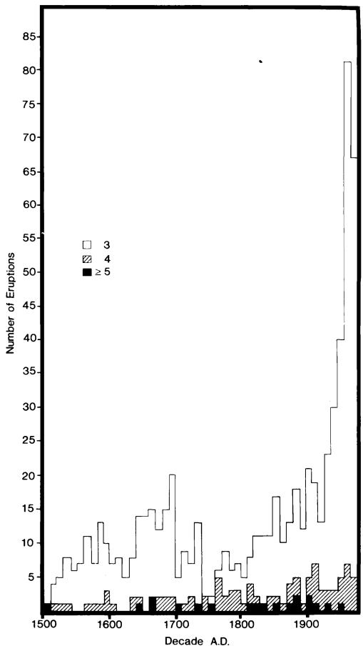
The Smithsonian Institution’s Global Volcanism Program (GVP) database, which catalogs 1,408 Holocene volcanoes and 9,928 eruptions, provides the foundational data for such analyses, yet the completeness of this record varies significantly by era and eruption magnitude. [181] As noted by Newhall and Self, the relative completeness of eruption dates only begins around 1800 for Volcanic Explosivity Index (VEI) ≥ 5 events, around 1900 for VEI = 4, and around 1960 for VEI = 3. [215] This temporal bias means that the striking increase in recorded VEI = 3 eruptions since 1800 likely reflects the progressive improvement in observing and reporting smaller eruptions, rather than an actual increase in worldwide volcanism. [215] Consequently, the historical record is spotty, especially for the period before the sixteenth century, and any analysis of long-term trends must account for these data gaps. When examining the annual frequency of eruptions from 1700 to 2020, researchers have applied smoothing filters to eliminate random variations, assuming that data gaps are a random process. [166] However, the incompleteness of the pre-modern record implies that many significant eruptions may have gone unrecorded or remain unknown to science. This uncertainty is critical when projecting future hazards. [82] Consequently, establishing these geological baselines indicates the potential for future large-scale eruptions to coincide with solar minima, highlighting the critical need for rigorous hazard assessment in regions like Peru where populations reside near active volcanic structures.
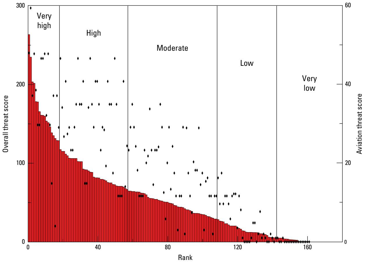
Attributing climate change to specific volcanic eruptions is challenging due to competing natural variability factors like solar radiation and oceanic oscillations. For instance, the massive Icelandic Laki eruption of June–August 1783 did not produce prompt apparent global cooling, likely because a strong El Niño event in 1782–1783 acted as an unknown moderating factor that diluted the volcanic signal. [287][215][49][76][1] Although large enough eruptions can poke through this variability to produce discernible effects in climatically sensitive regions like Europe, the need to treat each volcanic eruption on an individual basis remains critical. [287] Fumarolic activity had probably remained mild for at least tens of years, as historical accounts report that Indian people used to climb and perform offerings to Huaynaputina prior to AD 1600 with the aim of appeasing its activity. [256] The small amount of lithic fragments in the AD 1600 pumice-fall deposit indicates that the vent was already open in the amphitheater’s floor prior to the eruption, allowing the plinian column to evolve quickly. [256] Without repeated experiences, the process whereby managers evolve measures of coping with disasters does not take place. [39] The National Hurricane Center confirmed this insight after the 2004 and 2005 hurricane seasons, noting that those who have ‘never experienced a direct hit by a major hurricane’ seem incapable of envisaging what one is like. [39] Furthermore, those who have experienced such events ‘only remember the worst effects of a hurricane for about seven years.’ Consequently, predictions that the risk of a significant event is substantial do not, historically, generate the collective will necessary for us to make investments in resiliency. This holds true even when science indicates quite clearly that the event is quite likely to happen eventually and that the consequences of being unprepared will be severe. [39] As Clive Hamilton observed, ‘Sometimes facing up to the truth is just too hard. [39] When the facts are distressing it is easier to reframe or ignore them.’ [39] Geological Survey national volcanic threat assessment demonstrates the utility of this kind of risk analysis by ranking volcanoes into five relative threat groupings based on a 24-factor schema. [288] This methodology accounts for the highly variable knowledge of eruptive histories of more than 160 active U.S. volcanoes, as well as the diversity of eruptive styles and geographic settings. [288] By prioritizing where to focus volcanic risk mitigation through research, monitoring, hazard assessment, and community engagement, the framework serves as an effective communication tool for engaging stakeholders and the public. [288] The adaptation of this threat assessment methodology by groups in Chile, New Zealand, Argentina, the Caribbean region, and Peru, along with its inclusion in the United Nations Office for Disaster Risk Reduction Global Assessment Report for Risk Reduction 2015, suggests the broad applicability of such structured risk management frameworks. [288]
Modeling extreme volcanic events remains difficult because the information needed to constrain the frequency of outliers in probability distributions is often lacking. The frequency data for past volcanism has significant shortcomings and is generally incomplete, as noted by Newhall and Self. [289][166][215][290][291][257] While the decadal rate of all eruptions recorded in ice cores has remained approximately uniform for the last 1000 years, eruptive frequency estimates from other sources show a marked increase as they approach the present. [289] This apparent rise is largely attributed to the advent of satellite observations, which were able to catalogue smaller eruptions globally, rather than an actual increase in worldwide volcanism. [289] Extensive ice core samples reflect the occurrence of large eruptions but fail to capture the small ones. [289] Conversely, recent short-term observations accurately represent small, more frequent eruptions, but the repose times of the larger eruptions are beyond the length of the record. [289] Consequently, the relative frequencies of eruptions for the period 0–999 AD are much less than for the period 1000–2000 AD, leaving it unclear whether this reflects an actual lull in volcanism or a failure of the record to capture or preserve the events.
The geological record of Vesuvius reveals that prehistoric eruptions, specifically the Pomici di Base and Avellino Pumice events occurring 22,000 and 4,300 years ago respectively, were accompanied by debris avalanches that reached the coast. [82] This historical evidence suggests that future large-scale flank failures of volcanoes like Vesuvius raise implications for tsunami hazards associated with debris avalanches reaching the coast. Structural failure of the volcanic edifice could also occur, triggering landslides and potentially caldera formation, while mixing of ground water and magma within the conduit during the waning stages of an eruption could produce hydrovolcanic explosions. [82][288][272] The difficulty of reconciling purely statistical analyses of eruption frequency and clustering with what the geological record tells us about magma-reservoir processes means no one knows when Vesuvius will reawaken. [82] The 2018 update to the U.S. [288] This assessment framework underscores the need to monitor specific physical indicators, such as whether a volcano has produced a tsunami within the Holocene or has hydrothermal explosion potential due to extensive thermal features. [288]